How To Code RNN And LSTM Neural Networks In Python
import matplotlib.pyplot as plt
import numpy as np
import pandas as pd
import tensorflow as tf
from tensorflow import keras
from tensorflow.keras import layers

tf.__version__
Check out following links if you want to learn more about Pandas and Numpy.
What's so special about text?
Text is categorized as Sequential data: a document is a sequence of sentences, each sentence is a sequence of words, and each word is a sequence of characters. What is so special about text is that the next word in a sentence depends on:
- Context: which can extend long distances before and after the word, aka long term dependancy.
- Intent: different words can fit in the same contexts depending on the author's intent.
What do we need?
We need a neural network that models sequences. Specifically, given a sequence of words, we want to model the next word, then the next word, then the next word, ... and so on. That could be on a sentence, word, or character level. Our goal can be to just make a model to predict/generate the next word, like in unsupervised word embeddings. Alternatively, we could just map patterns in the text to associated labels, like in text classifications. In this notebook, we will be focusing on the latter. However, the networks used for either are pretty similar. The role of the network is most important in processing the textual input, extracting, and modelling the linguistic features. What we then do with these features is another story.
Recurrent Neural Networks (RNNs)
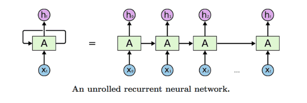
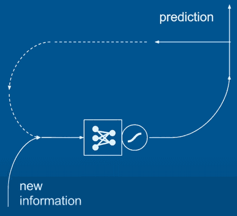
A Recurrent Neural Network (RNN) has a temporal dimension. In other words, the prediction of the first run of the network is fed as an input to the network in the next run. This beautifully reflects the nature of textual sequences: starting with the word "I" the network would expect to see "am", or "went", "go" ...etc. But then when we observe the next word, which let us say, is "am", the network tries to predict what comes after "I am", and so on. So yeah, it is a generative model!
Reber Grammar Classification
Let's start by a simple grammar classification. We assume there is a linguistic rule that characters are generated according to. This is a simple simulation of grammar in our natural language: you can say "I am" but not "I are". More onto Reber Grammar > here.
Defining the grammar
Consider the following Reber Grammar:
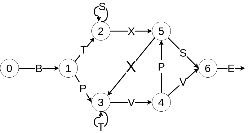
Let's represent it first in Python:
default_reber_grammar=[
    [("B",1)],  #(state 0) =B=> (state 1)
    [("T", 2),("P", 3)],  # (state 1) =T=> (state 2) or =P=> (state 3)
    [("X", 5), ("S", 2)], # (state 2) =X=> (state 5) or =S=> (state 2)
    [("T", 3), ("V", 4)], # (state 3) =T=> (state 3) or =V=> (state 4)
    [("V", 6), ("P", 5)], # (state 4) =V=> (state 6) or =P=> (state 5)
    [("X",3), ("S", 6)],  # (state 5) =X=> (state 3) or =S=> (state 6)
    [("E", None)]         # (state 6) =E=> <EOS>

]
Let's take this a step further, and use Embedded Reber Grammar, which simulates slightly more complicated linguistic rules, such as phrases!
embedded_reber_grammar=[
    [("B",1)],  #(state 0) =B=> (state 1)
    [("T", 2),("P", 3)],  # (state 1) =T=> (state 2) or =P=> (state 3)
    [(default_reber_grammar,4)], # (state 2) =REBER=> (state 4)
    [(default_reber_grammar,5)], # (state 3) =REBER=> (state 5)
    [("P", 6)], # (state 4) =P=> (state 6)
    [("T",6)],  # (state 5) =T=> (state 3)
    [("E", None)]         # (state 6) =E=> <EOS>

]
Now let's generate some data using these grammars:
def generate_valid_string(grammar):
    state = 0
    output = []
    while state is not None:
        char, state = grammar[state][np.random.randint(len(grammar[state]))]
        if isinstance(char, list):  # embedded reber
            char = generate_valid_string(char)
        output.append(char)
    return "".join(output)
def generate_corrupted_string(grammar, chars='BTSXPVE'):
    '''Substitute one character to violate the grammar'''
    good_string = generate_valid_string(grammar)
    idx = np.random.randint(len(good_string))
    good_char = good_string[idx]
    bad_char = np.random.choice(sorted(set(chars)-set(good_char)))
    return good_string[:idx]+bad_char+good_string[idx+1:]
Let's define all the possible characters used in the grammar.
chars='BTSXPVE'
chars_dict = {a:i for i,a in enumerate(chars)}
chars_dict
One hot encoding is used to represent each character with a vector so that all vectors are equally far away from each other. For example,
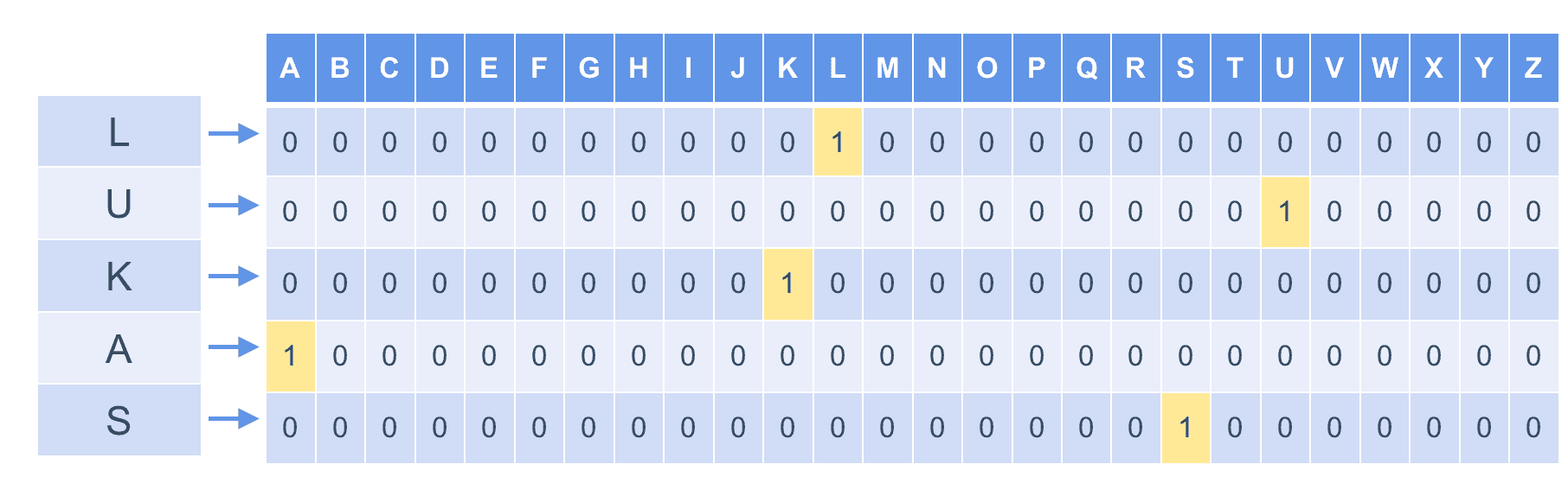
def str2onehot(string, num_steps=12, chars_dict=chars_dict):
    res = np.zeros((num_steps, len(chars_dict)))
    for i in range(min(len(string), num_steps)):
        c = string[i]
        res[i][chars_dict[c]] = 1
    return res
Now let's generate a dataset of valid and corrupted strings
def generate_data(data_size=10000, grammar=embedded_reber_grammar, num_steps=None):
    good = [generate_valid_string(grammar) for _ in range(data_size//2)]
    bad = [generate_corrupted_string(grammar) for _ in range(data_size//2)]
    all_strings = good+bad
    if num_steps is None:
        num_steps = max([len(s) for s in all_strings])
    X = np.array([str2onehot(s) for s in all_strings])
    l = np.array([len(s) for s in all_strings])
    y = np.concatenate((np.ones(len(good)), np.zeros((len(bad))))).reshape(-1, 1)
    idx = np.random.permutation(data_size)
    return X[idx], l[idx], y[idx]
np.random.seed(42)
X_train, seq_lens_train, y_train = generate_data(10000)
X_val, seq_lens_val, y_val = generate_data(5000)
X_train.shape, X_val.shape
We have 10,000 words, each with 12 characters, and maximum of 7 unique letters (i.e. BTSXPVE)
source
x = layers.Input(shape=(12, 7)) # we define our input's shape
# first we define our RNN cells to use in the RNN model
# let's keep the model simple ...
cell = layers.SimpleRNNCell(4, activation='tanh')  # ... by just using 4 units (like 4 units in hidden layers)
rnn = layers.RNN(cell)
rnn_output = rnn(x)
We use tanh activation function to make the prediction between -1 and 1 the resulting activation between -1 and 1 is then weighted to finally give us the features to use in making our predictions
We finally add a fully connected layer to map our rnn outputs to the 0-1 classification output. We use a sigmoid function to map the prediction to probabilities between 0 and 1.
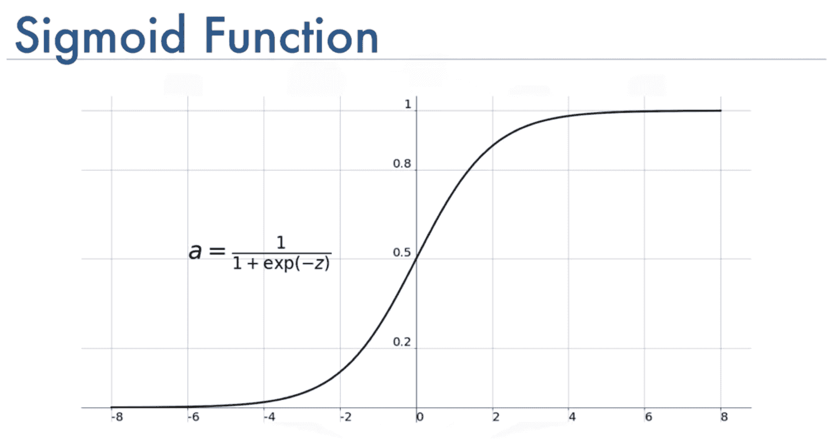
output = layers.Dense(units=1, activation='sigmoid')(rnn_output)
# let's compile the model
model = keras.Model(inputs=x, outputs=output)
# loss is binary cropss entropy since this is a binary classification task
# and evaluation metric as f1
model.compile(loss="binary_crossentropy", metrics=["accuracy"])
model.summary()
We have 12 characters in each input, and 4 units per RNN cell, so we have a total of 12x4=48 parameters to learn + 5 more parameters from the fully connected (FC) layer.
# we train the model for 100 epochs
# verbose level 2 displays more info while trianing
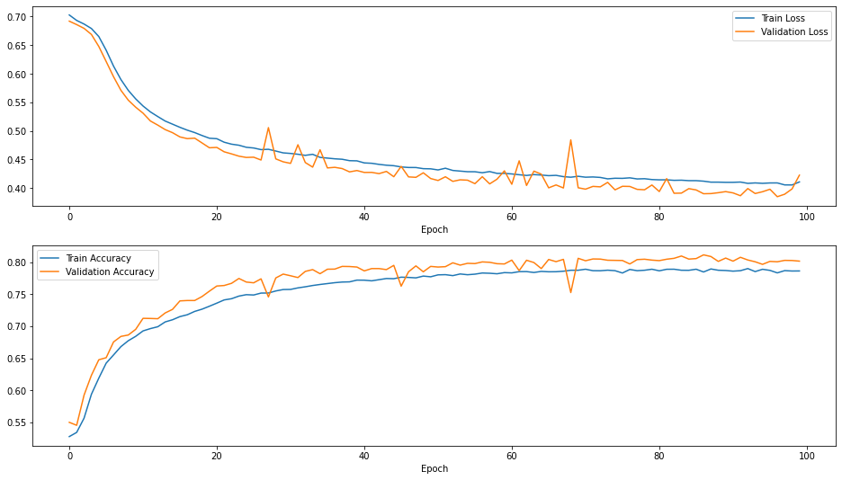
H = model.fit(X_train, y_train, epochs=100, verbose=2, validation_data=(X_val, y_val))
def plot_results(H):
    results = pd.DataFrame({"Train Loss": H.history['loss'], "Validation Loss": H.history['val_loss'],
              "Train Accuracy": H.history['accuracy'], "Validation Accuracy": H.history['val_accuracy']
             })
    fig, ax = plt.subplots(nrows=2, figsize=(16, 9))
    results[["Train Loss", "Validation Loss"]].plot(ax=ax[0])
    results[["Train Accuracy", "Validation Accuracy"]].plot(ax=ax[1])
    ax[0].set_xlabel("Epoch")
    ax[1].set_xlabel("Epoch")
    plt.show()
plot_results(H)
LSTM
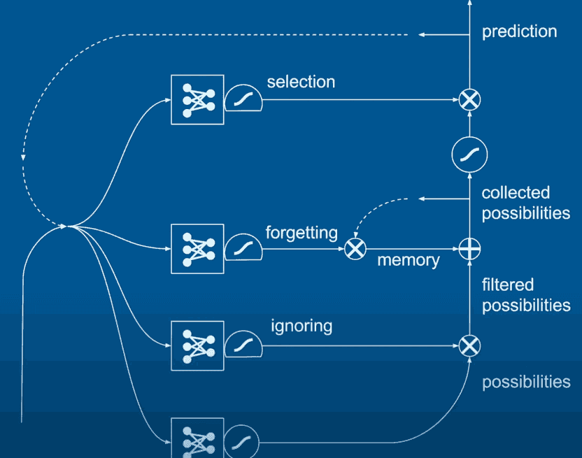
Long short-term memory employs logic gates to control multiple RNNs, each is trained for a specific task. LSTMs allow the model to memorize long-term dependancies and forget less likely predictions. For example, if the training data had "John saw Sarah" and "Sarah saw John", when the model is given "John saw", the word "saw" can predict "Sarah" and "John" as they have been seen just after "saw". LSTM allows the model to recognize that "John saw" is going to undermine the possibility for "John", so we won't get "John saw John". Also we won't get "John saw John saw John saw John ..." as the model can predict that what comes after the word after saw, is the end of the sentence.
source
Now we will apply bidirectional LSTM (that looks both backward and forward in the sentence) for text classification.
!pip install -q tensorflow_datasets
import tensorflow_datasets as tfds
dataset, info = tfds.load('imdb_reviews', with_info=True,
                          as_supervised=True)
train_dataset, test_dataset = dataset['train'], dataset['test']
train = train_dataset.take(4000)
test = test_dataset.take(1000)
# to shuffle the data ...
BUFFER_SIZE = 4000 # we will put all the data into this big buffer, and sample randomly from the buffer
BATCH_SIZE = 128  # we will read 128 reviews at a time

train = train.shuffle(BUFFER_SIZE).batch(BATCH_SIZE)
test = test.batch(BATCH_SIZE)
prefetch: to allow the later elements to be prepared while the current elements are being processed.
train = train.prefetch(BUFFER_SIZE)
test = test.prefetch(BUFFER_SIZE)
VOCAB_SIZE=1000 # assuming our vocabulary is just 1000 words

encoder = layers.experimental.preprocessing.TextVectorization(max_tokens=VOCAB_SIZE)

encoder.adapt(train.map(lambda text, label: text)) # we just encode the text, not the labels
# here are the first 20 words in our 1000-word vocabulary
vocab = np.array(encoder.get_vocabulary())
vocab[:20]
example, label = list(train.take(1))[0] # that's one batch
len(example)
example[0].numpy()
encoded_example = encoder(example[:1]).numpy()
encoded_example
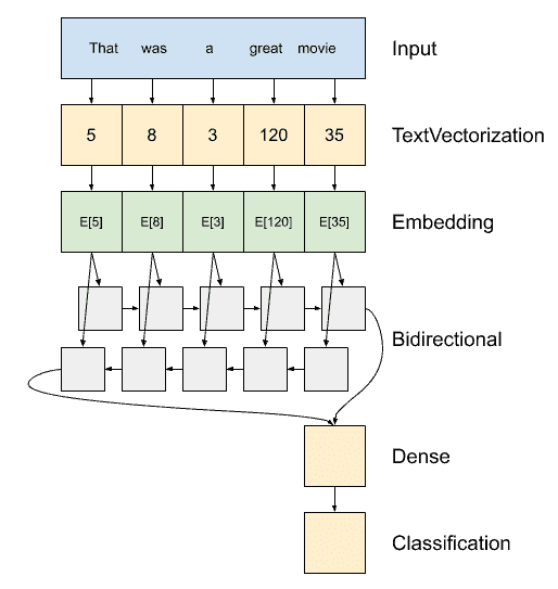
model = tf.keras.Sequential([
    encoder, # the encoder
    tf.keras.layers.Embedding(
        input_dim=len(encoder.get_vocabulary()),
        output_dim=64,
        # Use masking to handle the variable sequence lengths
        mask_zero=True),
    tf.keras.layers.Bidirectional(layers.LSTM(64)), # making LSTM bidirectional
    tf.keras.layers.Dense(32, activation='relu'), # FC layer for the classification part
    tf.keras.layers.Dense(1) # final FC layer

])
Let's try it out!
sample_text = ('The movie was cool. The animation and the graphics '
               'were out of this world. I would recommend this movie.')
predictions = model.predict(np.array([sample_text]))
print(predictions[0])
yeah yeah, we haven't trained the model yet.
# we will use binary cross entropy again because this is a binary classification task (positive or negative)
# we also did not apply a sigmoid activation function at the last FC layer, so we specify that the
# are calculating the cross entropy from logits
model.compile(
    loss=tf.keras.losses.BinaryCrossentropy(from_logits=True),
    # adam optimizer is more efficient (not always the most accurate though)
    optimizer=tf.keras.optimizers.Adam(1e-4),
    metrics=['accuracy']
)
model.summary()
Wow that's a lot of parameters!
H2 = model.fit(train, epochs=25,
                    validation_data=test)
plot_results(H2)
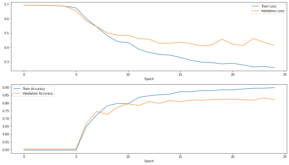
It works! We stopped after only 25 epochs, but obviously still has plenty of room for fitting with more epochs.
Summary & Comments
- Text is a simply a sequential data.
- RNN-like models feed the prediction of the current run as input to the next run.
- LSTM uses 4 RNNs to handel more complex features of text (e.g. long-term dependancy)
- Bidirectional models can provide remarkably outperform unidirectional models.
- You can stack as many LSTM layers as you want. It is just a new LEGO piece to use when building your NN :)
Related Notebooks
- Activation Functions In Artificial Neural Networks Part 2 Binary Classification
- Learn And Code Confusion Matrix With Python
- Rectified Linear Unit For Artificial Neural Networks Part 1 Regression
- How To Run Code From Git Repo In Collab GPU Notebook
- Generative Adversarial Networks
- How to do SQL Select and Where Using Python Pandas
- Strftime and Strptime In Python
- Tweet Sentiment Analysis Using LSTM With PyTorch
- How to Plot a Histogram in Python