Understanding Autoencoders With Examples

Introduction to Autoencoders

The idea about autoencoders is pretty straight forward. Predict what you input.

  • What is the point then? Well, we know that neural networks (NNs) are just a sequence of matrix multiplications. Let's say the shape of the input matrix is (n, k), which means there are n instances with k features. We want to predict a single output for each of the n instances, that is (n, 1). So we can simply multiply the (n, k) matrix by a (k, 1) matrix to get a (n, 1) matrix. The (n, 1) matrix resulting from this multiplication is then compared with the (n, 1) labels, where the error is used to optimize the (k, 1). But are we really limited to a single (k, 1) matrix? Not at all! We can have much longer sequences, for example:

    • Input: (n, k) x (k, 100) x (100, 50) x (50, 20) x (20, 1) ==> (n, 1): Output These intermediary matrices between the input and the output layers are the hidden layers of the neural network. These hidden layers hold latent information about the representation of the input data. For example, if the input is a flattened image. Let's say the image is 800x600 pixels, that's a total of 480,000 pixels. That's a lot of features! But immediately after the first hidden layer (k, 100), that image gets compressed into only 100 dimensions! Why don't we use this magic hidden layer then to reduce the dimensionilty of high-dimensional data, like images or text. Yes, text can be very high dimensional if you want to use one-hot encoding for words in data that has +100k words!

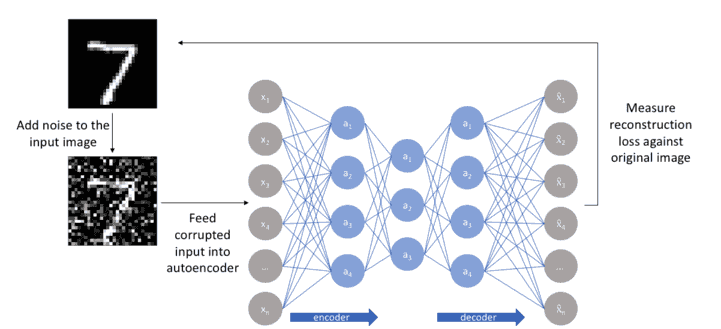
  • What can we make out of this then? Give the input to a hidden layer (or layers) and let the output be exactly the same as shape as the input. The goal would be to reproduce the input after multiplying the input with these hidden layers. So basically we compress the input and then decompress it. Or rather, we encode the input then decode it, hence the name autoencoder. Auto because it requires only the input to encode and decode it. And encoder is for the compression/encoding part.

  • Where is that useful? This compressed representation of the input has many cool usages:
    1. Dimensionality Reduction. Your memory will pray for you!
    2. Image-to-image translation.
    3. Denoising.
    4. Text Representation

Dimensionality Reduction

Autoencoders learn non-linear transformations, making them better than PCA for dimensionality reduction. Check out these results:

PCA works with linear transformations, so it works with flat surfaces or lines. Autoencoders use activation functions since it is a neural network afterall, so it can model non-linear transformations.

Image-to-image translation

Being compressed, it can be used as an intermediary step (often called a latent space) to transform the input. If you have two images of the same person. One image is with that person wearing glasses, and the other without. If the autoencoder is trained to encode this image, it can be also trained to decode the image with glasses to an image without glasses! Same goes for adding a beard, or making someone blonde. You get the idea. This is called image-to-image transformation, and it requires some tweaking for the network. Here is a slightly different example:

Denoising

By deliberately adding noise to the input, autoencoders can be trained to reconstruct the original image before adding noise. Since the input and the target output are no longer the same, autoencoders do not just memorize the training data.

Text-representation

The hidden layer the autoencoder that compresses the input in is actually an embedding! You can call it a latent space, a hidden layer, or an embedding. So, the autoencoder converts the data into an embedding.

Did someone just say embeddings? Yes! we can use autoencoders to learn word embeddings. Let's now do that in Keras.

Check out following links to learn more about word embeddings...

https://www.nbshare.io/notebook/595607887/Understanding-Word-Embeddings-Using-Spacy-Python/

https://www.nbshare.io/notebook/197284676/Word-Embeddings-Transformers-In-SVM-Classifier-Using-Python/

Keras Implementation

The embedding layer

The Embedding layer in keras takes three arguments:

  • input_dim: The size of the input vectors. In our case, the size of the vocabulary.
  • output_dim: The size of the output vectors. Basically, how many dimensions do you want to compress the data into?\
  • input_length: The length of input sequences. In our cases, the maximum number of words in a sentence.

Data

In [1]:
import numpy as np
In [2]:
docs = [
    "Beautifully done!",
    "Excellent work",
    "Admirable effort",
    "Satisfactory performance",
    "very bad",
    "unacceptable results",
    "incompetent with poor skills",
    "not cool at all"
]
# let's make this a sentiment analysis task!
labels = np.array([1, 1, 1, 1, 0, 0, 0, 0])
In [3]:
# vocabulary
# by iterating on each document and fetching each word, and converting it to a lower case
# then removing duplicates by converting the resulting list into a set
vocab = set([w.lower() for doc in docs for w in doc.split()])
vocab
Out[3]:
{'admirable',
 'all',
 'at',
 'bad',
 'beautifully',
 'cool',
 'done!',
 'effort',
 'excellent',
 'incompetent',
 'not',
 'performance',
 'poor',
 'results',
 'satisfactory',
 'skills',
 'unacceptable',
 'very',
 'with',
 'work'}
In [4]:
vocab_size = len(vocab)
vocab_size
Out[4]:
20
In [5]:
# one-hot encoding
from keras.preprocessing.text import one_hot
encoded_docs = [one_hot(d, vocab_size) for d in docs]
# this will convert sentences into a list of lists with indices of each word in the vocabulary
encoded_docs
Out[5]:
[[10, 10],
 [19, 15],
 [1, 2],
 [9, 9],
 [1, 2],
 [4, 11],
 [19, 11, 7, 7],
 [12, 13, 1, 5]]
In [6]:
# getting the maximum number of words in a sentence in our data
max_length = max([len(doc.split()) for doc in docs])
max_length
Out[6]:
4
In [7]:
from keras.preprocessing.sequence import pad_sequences
# padding sentences with words less than max_length to make all input sequences with the same size
padded_docs = pad_sequences(encoded_docs, maxlen=max_length, padding='post')
padded_docs
Out[7]:
array([[10, 10,  0,  0],
       [19, 15,  0,  0],
       [ 1,  2,  0,  0],
       [ 9,  9,  0,  0],
       [ 1,  2,  0,  0],
       [ 4, 11,  0,  0],
       [19, 11,  7,  7],
       [12, 13,  1,  5]], dtype=int32)

Model

In [8]:
from keras.layers import Dense, Flatten
from keras.layers.embeddings import Embedding
from keras.models import Sequential
In [9]:
model = Sequential()
model.add(Embedding(input_dim=vocab_size, output_dim=8, input_length=max_length))
model.add(Flatten())
model.add(Dense(1, activation='sigmoid')) # we are using sigmoid here since this is a binary classification task

model.compile(optimizer='adam', loss='binary_crossentropy', metrics=['accuracy'])

model.summary()
Model: "sequential"
_________________________________________________________________
Layer (type)                 Output Shape              Param #   
=================================================================
embedding (Embedding)        (None, 4, 8)              160       
_________________________________________________________________
flatten (Flatten)            (None, 32)                0         
_________________________________________________________________
dense (Dense)                (None, 1)                 33        
=================================================================
Total params: 193
Trainable params: 193
Non-trainable params: 0
_________________________________________________________________
In [10]:
import matplotlib.pyplot as plt
In [11]:
H = model.fit(padded_docs, labels, epochs=50)
Epoch 1/50
1/1 [==============================] - 0s 401ms/step - loss: 0.7077 - accuracy: 0.2500
Epoch 2/50
1/1 [==============================] - 0s 1ms/step - loss: 0.7058 - accuracy: 0.2500
Epoch 3/50
1/1 [==============================] - 0s 1ms/step - loss: 0.7039 - accuracy: 0.2500
Epoch 4/50
1/1 [==============================] - 0s 1ms/step - loss: 0.7019 - accuracy: 0.2500
Epoch 5/50
1/1 [==============================] - 0s 1ms/step - loss: 0.7000 - accuracy: 0.2500
Epoch 6/50
1/1 [==============================] - 0s 2ms/step - loss: 0.6982 - accuracy: 0.3750
Epoch 7/50
1/1 [==============================] - 0s 1ms/step - loss: 0.6963 - accuracy: 0.3750
Epoch 8/50
1/1 [==============================] - 0s 1ms/step - loss: 0.6944 - accuracy: 0.3750
Epoch 9/50
1/1 [==============================] - 0s 1ms/step - loss: 0.6925 - accuracy: 0.5000
Epoch 10/50
1/1 [==============================] - 0s 1ms/step - loss: 0.6907 - accuracy: 0.6250
Epoch 11/50
1/1 [==============================] - 0s 2ms/step - loss: 0.6888 - accuracy: 0.6250
Epoch 12/50
1/1 [==============================] - 0s 1ms/step - loss: 0.6870 - accuracy: 0.7500
Epoch 13/50
1/1 [==============================] - 0s 1ms/step - loss: 0.6851 - accuracy: 0.7500
Epoch 14/50
1/1 [==============================] - 0s 1ms/step - loss: 0.6833 - accuracy: 0.8750
Epoch 15/50
1/1 [==============================] - 0s 2ms/step - loss: 0.6814 - accuracy: 0.8750
Epoch 16/50
1/1 [==============================] - 0s 1ms/step - loss: 0.6796 - accuracy: 0.8750
Epoch 17/50
1/1 [==============================] - 0s 1ms/step - loss: 0.6777 - accuracy: 0.8750
Epoch 18/50
1/1 [==============================] - 0s 1ms/step - loss: 0.6759 - accuracy: 0.8750
Epoch 19/50
1/1 [==============================] - 0s 1ms/step - loss: 0.6741 - accuracy: 0.8750
Epoch 20/50
1/1 [==============================] - 0s 1ms/step - loss: 0.6722 - accuracy: 0.8750
Epoch 21/50
1/1 [==============================] - 0s 1ms/step - loss: 0.6704 - accuracy: 0.8750
Epoch 22/50
1/1 [==============================] - 0s 1ms/step - loss: 0.6685 - accuracy: 0.8750
Epoch 23/50
1/1 [==============================] - 0s 2ms/step - loss: 0.6667 - accuracy: 0.8750
Epoch 24/50
1/1 [==============================] - 0s 1ms/step - loss: 0.6648 - accuracy: 0.8750
Epoch 25/50
1/1 [==============================] - 0s 1ms/step - loss: 0.6630 - accuracy: 0.8750
Epoch 26/50
1/1 [==============================] - 0s 2ms/step - loss: 0.6611 - accuracy: 0.8750
Epoch 27/50
1/1 [==============================] - 0s 1ms/step - loss: 0.6593 - accuracy: 0.8750
Epoch 28/50
1/1 [==============================] - 0s 1ms/step - loss: 0.6574 - accuracy: 0.8750
Epoch 29/50
1/1 [==============================] - 0s 1ms/step - loss: 0.6556 - accuracy: 0.8750
Epoch 30/50
1/1 [==============================] - 0s 1ms/step - loss: 0.6537 - accuracy: 0.8750
Epoch 31/50
1/1 [==============================] - 0s 1ms/step - loss: 0.6518 - accuracy: 0.8750
Epoch 32/50
1/1 [==============================] - 0s 1ms/step - loss: 0.6499 - accuracy: 0.8750
Epoch 33/50
1/1 [==============================] - 0s 1ms/step - loss: 0.6480 - accuracy: 0.8750
Epoch 34/50
1/1 [==============================] - 0s 1ms/step - loss: 0.6462 - accuracy: 0.8750
Epoch 35/50
1/1 [==============================] - 0s 1ms/step - loss: 0.6443 - accuracy: 0.8750
Epoch 36/50
1/1 [==============================] - 0s 1ms/step - loss: 0.6423 - accuracy: 0.8750
Epoch 37/50
1/1 [==============================] - 0s 1ms/step - loss: 0.6404 - accuracy: 0.8750
Epoch 38/50
1/1 [==============================] - 0s 1ms/step - loss: 0.6385 - accuracy: 0.8750
Epoch 39/50
1/1 [==============================] - 0s 1ms/step - loss: 0.6366 - accuracy: 0.8750
Epoch 40/50
1/1 [==============================] - 0s 1ms/step - loss: 0.6346 - accuracy: 0.8750
Epoch 41/50
1/1 [==============================] - 0s 1ms/step - loss: 0.6327 - accuracy: 0.8750
Epoch 42/50
1/1 [==============================] - 0s 2ms/step - loss: 0.6307 - accuracy: 0.8750
Epoch 43/50
1/1 [==============================] - 0s 1ms/step - loss: 0.6287 - accuracy: 0.8750
Epoch 44/50
1/1 [==============================] - 0s 1ms/step - loss: 0.6268 - accuracy: 0.8750
Epoch 45/50
1/1 [==============================] - 0s 1ms/step - loss: 0.6248 - accuracy: 0.8750
Epoch 46/50
1/1 [==============================] - 0s 1ms/step - loss: 0.6228 - accuracy: 0.8750
Epoch 47/50
1/1 [==============================] - 0s 1ms/step - loss: 0.6208 - accuracy: 0.8750
Epoch 48/50
1/1 [==============================] - 0s 1ms/step - loss: 0.6187 - accuracy: 0.8750
Epoch 49/50
1/1 [==============================] - 0s 1ms/step - loss: 0.6167 - accuracy: 0.8750
Epoch 50/50
1/1 [==============================] - 0s 1ms/step - loss: 0.6146 - accuracy: 0.8750
In [12]:
fig,ax = plt.subplots(figsize=(16, 9))
ax.plot(H.history["loss"], label="loss", color='r')
ax.set_xlabel("Epoch", fontsize=15)
ax.set_ylabel("Loss", fontsize=15)
ax2 = ax.twinx()
ax2.plot(H.history["accuracy"], label="accuracy", color='b')
ax2.set_ylabel("Accuracy", fontsize=15)
plt.legend()
plt.show()
In [13]:
loss, accuracy = model.evaluate(padded_docs, labels, verbose=0)
print(f'Accuracy: {round(accuracy*100, 2)}')
Accuracy: 87.5
In [14]:
from sklearn.metrics import classification_report
In [15]:
y_pred = model.predict(padded_docs)>0.5
y_pred
Out[15]:
array([[ True],
       [ True],
       [ True],
       [ True],
       [ True],
       [False],
       [False],
       [False]])

Let us print the confusion matrix

In [16]:
print(classification_report(labels, y_pred))
              precision    recall  f1-score   support

           0       1.00      0.75      0.86         4
           1       0.80      1.00      0.89         4

    accuracy                           0.88         8
   macro avg       0.90      0.88      0.87         8
weighted avg       0.90      0.88      0.87         8