Understanding Word Embeddings Using Spacy Python
In this post, we will go over "What are Word Embeddings" and how to generate Word embeddings for stock tweets using Python package Spacy.
!pip install spacy
To download pre-trained models for English:
!spacy download en_core_web_lg
!pip install tweet-preprocessor
Ok for this post, we will use stock tweets data. For data analyzing, we will use Python package pandas.
Let us look at our data first.
import pandas as pd
df = pd.read_csv("stocktweets/tweets/stocktwits.csv")
df.head(2)
Cleaning the data
We use `tweet-preprocessor`
pip install tweet-preprocessor
The following code will do...
- Remove mentions and URLs
- Remove non-alphanumeric characters
- Rgnores Sentences with less than 3 words
- Lower case everything
- Remove redundant spaces
import re
import string

import preprocessor as p
from spacy.lang.en import stop_words as spacy_stopwords

p.set_options(p.OPT.URL, p.OPT.MENTION)  # removes mentions and URLs only
stop_words = spacy_stopwords.STOP_WORDS
punctuations = string.punctuation


def clean(text):
    text = p.clean(text)
    text = re.sub(r'\W+', ' ', text)  # remove non-alphanumeric characters
    # replace numbers with the word 'number'
    text = re.sub(r"\d+", "number", text)
    # don't consider sentenced with less than 3 words (i.e. assumed noise)
    if len(text.strip().split()) < 3:
        return None
    text = text.lower()  # lower case everything

    return text.strip() # remove redundant spaces
Ok let us now remove the na using dropna()
df = df.assign(clean_text=df.message.apply(clean)).dropna()
df.head(2)
from IPython.display import Image
Image(filename="images/spacy_word_embeddings.png")
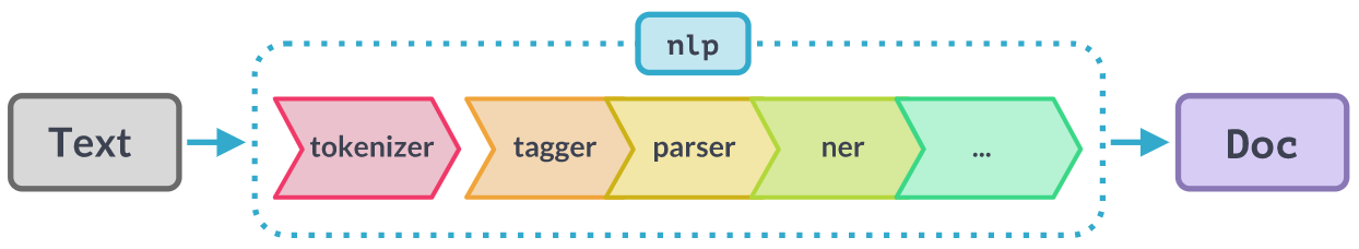
import spacy
nlp = spacy.load("en_core_web_lg") # loading English data
# for example
hello = nlp("hello")
hello.vector.shape # we get a 300-dimensional vector representing the word hello
Image(filename="images/tokenization.png")
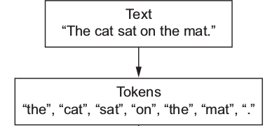
Let us initialize our NLP tokenizer.
# first we define our tokenizer
spacy_tokenizer = nlp.tokenizer
list(spacy_tokenizer("hello how are you"))
Image(filename="images/lemmatization.png")
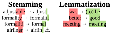
For simplicity we will just assume that each tweet is one sentence. Below tokenize function does lemmatization and remove stop words.
def tokenize(sentence):
    sentence = nlp(sentence)
    # lemmatizing
    sentence = [ word.lemma_.lower().strip() if word.lemma_ != "-PRON-" else word.lower_ for word in sentence ]
    # removing stop words
    sentence = [ word for word in sentence if word not in stop_words and word not in punctuations ]
    return sentence
Let us apply the tokenize function on a arbitrary sentence.
tokenize("hello how are you this is a very interesting topic")
Let us import tqdm and initialize to keep track of our code(run) progress.
from tqdm import tqdm
tqdm.pandas() # to keep track of our progress
Let us apply the tokenizer to our entire corpus first.
sentences = df.clean_text.progress_apply(tokenize) # first we get list of lists of tokens composing each sentence
# this process takes a while!
vocab = set()
for s in sentences:
    vocab.update(set(s))
vocab = list(vocab) # to make sure order matters
print(f"We have {len(vocab)} tokens in our vocab")
# this also takes a while, but it is slightly faster than tokenization
vectors=[]
for token in tqdm(vocab):
    vectors.append(nlp(token).vector)
Projecting The Word Vectors onto a 2D Plane
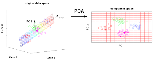
We use PCA to reduce the 300 dimensions of our word embeddins into just 2 dimensions. If your data is 3D, then PCA tries to find the best 2D plane to capture most information from the data. In our case, the data is 300D, and we are looking for the best 2D plane to represent our data on. Each axis of the 2D plane we are trying to find is Principal Component (PC), hence the name Principal Component Analysis; the process of analyzing the data and finding the best principal components to represent the data with much smaller number of dimensions.
Example:
Image(filename="images/pca.png")
PCA Using Sklearn
from sklearn.decomposition import PCA
The following code will transform our stock tweets data in to 2D data using sklearn principal component analysis.
pca = PCA(n_components=2)
embeddings_2d = pca.fit_transform(vectors)
I will use plolty to plot the word embeddings.
!pip install plotly
import plotly.express as px
from plotly.offline import init_notebook_mode
init_notebook_mode() # required to reload the figures upon re-opening the notebook
Before we do plotting, we need to convert our word embedding vectors in to Pandas DataFrame.
embeddings_df = pd.DataFrame({"x":embeddings_2d[:, 0], "y":embeddings_2d[:, 1], "token":vocab})
Below code will generate the scatter plot of our word embedding tokens.
fig = px.scatter(embeddings_df, x='x', y='y', opacity=0.5, hover_data=['token'])
fig.show()
Image(filename="images/embeddings_plot-min.png")
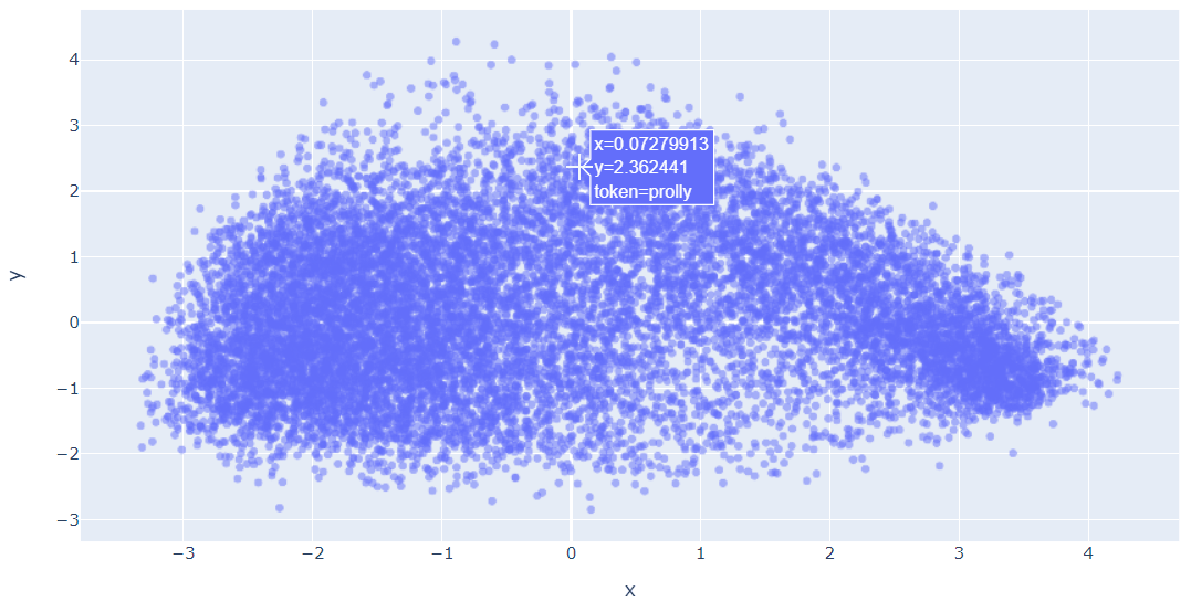
Not showing the plot because of size.
# you could also use matplotlib
import matplotlib.pyplot as plt

fig = plt.figure(figsize=(16, 9))

x_axis = embeddings_2d[:, 0]
y_axis = embeddings_2d[:, 1]

#plt.scatter(x_axis, y_axis, s=5, alpha=0.5) # alpha for transparency
#plt.show()
Not showing the plot because of size.
There we have it! Words represented numerically and even plotted on a 2D plane. Typically, if our dataset is sufficiently large, we can see words organized in a more meaningful way. We can even use these vectors to do word-math!
Image(filename="images/word_embeddings_meaning.png")
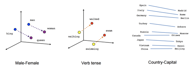
Notice that we are using a pre-trained model from Spacy, that was trained on a different dataset. So even though our dataset is pretty small we can still represent our tweets numerically with meaningful embeddings, that is, similar tweets are going to have similar (or closer) vectors, and dissimilar tweets are going to have very different (or distant) vectors.
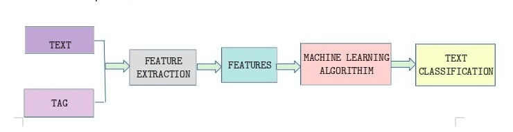
To check if we can use these embeddings to extract out any meaning from our stock tweets, we can use these as features in a downstream task, such as text classification.
Image(filename="images/text-classification-python-spacy.png")
Below code uses Sklearn's base class for transformers to fit and transform the data.
# we just make a data type that has the functions fit and transform
from sklearn.base import TransformerMixin
class SpacyEmbeddings(TransformerMixin): # it inherits the sklearn's base class for transformers
    def transform(self, X, **transform_params):
        # Cleaning Text
        return [sentence for sentence in X]

    def fit(self, X, y=None, **fit_params):
        return self

    def get_params(self, deep=True):
        return {}
From Word Embeddings to Sentence Embeddings
We simply can take the sum of word embedding vectors, in what is called the Bag of Words (BOW) approach.
For example,
- v1 = [1, 2, 3]
- v2 = [3, 4, 5]
- v3 = [5, 6, 7]
Assume that the sentence that has the vectors v1, v2, and v3.Then the sentence vector will be...
sentence_vector = [9, 12, 15]
Count vectorizer from Sklearn can be used to generate the sentence vectors. Counter Vectorization uses bag-of-word.
Below code uses CountVectorizer with Spacy tokenizer.
from sklearn.feature_extraction.text import CountVectorizer

bow_vector = CountVectorizer(tokenizer=spacy_tokenizer, ngram_range=(1,1))
Image(filename="images/Decision_Tree-2.png")
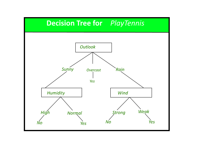
The problem is, our dataset is very imbalanced. There are way more "Bullish" tweets than "Bearish" tweets. So we need to let the classifier know about this so it doesn't just classify everything as "Bullish".
from sklearn.tree import DecisionTreeClassifier
from sklearn.model_selection import train_test_split
from sklearn.utils.class_weight import compute_class_weight
X, y = df["clean_text"], df["sentiment"]
# random_state ensures that whoever runs this notebook is going to get the same data split
X_train, X_test, y_train, y_test = train_test_split(X, y, random_state=42)
class_weight = compute_class_weight(
    class_weight='balanced', classes=["Bullish","Bearish"], y=y_train
)
class_weight
classifier = DecisionTreeClassifier(
    class_weight={"Bullish":class_weight[0], "Bearish":class_weight[1]}
)
Ok, let us build the model using Sklearn pipeline. The input to our pipeline will be "word embeddings", "vectorizer" and then a "classifier" in the same order.
from sklearn.pipeline import Pipeline # we use sklearn's pipeline
# Create pipeline using Bag of Words
pipe = Pipeline([("embedder", SpacyEmbeddings()),
                 ('vectorizer', bow_vector),
                 ('classifier', classifier)])

pipe.fit(X_train, y_train)
To evaluate the model, let us try using our classifer to predict sentiment on our test data.
predictions = pipe.predict(X_test)
Let us print our classification results.
from sklearn.metrics import classification_report
print(classification_report(y_test, predictions))
It seems the model is still tending to classify everyhing as Bullish, this could mean that we need a better classifier to detect the patterns in the tweets, especially that this is a very challenging task to address with a simple classifier as Decision Tree. Nevertheless, the embeddings have proven to be useful to be used in downstream tasks as a way to represent tweets.
Related Notebooks
- Word Embeddings Transformers In SVM Classifier Using Python
- Understanding Logistic Regression Using Python
- How to Generate Embeddings from a Server and Index Them Using FAISS with API
- Crawl Websites Using Python
- TTM Squeeze Stocks Scanner Using Python
- Demystifying Stock Options Vega Using Python
- How to Visualize Data Using Python - Matplotlib
- How To Read CSV File Using Python PySpark
- How To Read JSON Data Using Python Pandas