Word Embeddings Transformers In SVM Classifier Using Python
Word Embeddings
Word Embeddings is the process of representing words with numerical vectors.
One-hot-encoding
Not so long ago, words used to be represented numerically using sparse vectors that is all zeros except for the index of the corresponding word. For example, if we wanted to represent color words, ...
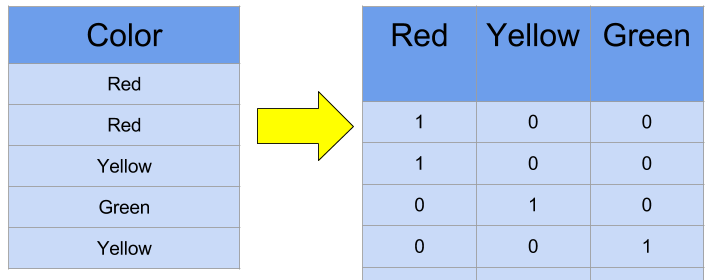
Problem with this approach is that all words are exactly the same distance from each other, so we cannot capture any semantic similarities with this approach. Also, with large vocabulary, the word vectors become extremely large, making that approach unefficient.
Static Word Embeddings (Word2Vec)
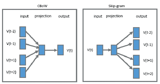
The idea about static word embeddings is to learn stand-alone vector representation of words from a text corpus. The goal was to estimate a dense low-dimensional vector representation of the words in a way that words similar in meaning should have vectors closer to each other than the vectors of words dissimilar in meaning. This came to be called word2vec, and it was trained using two variations, either using the context to predict a word (CBOW), or using a word to predict its context (SkipGram).
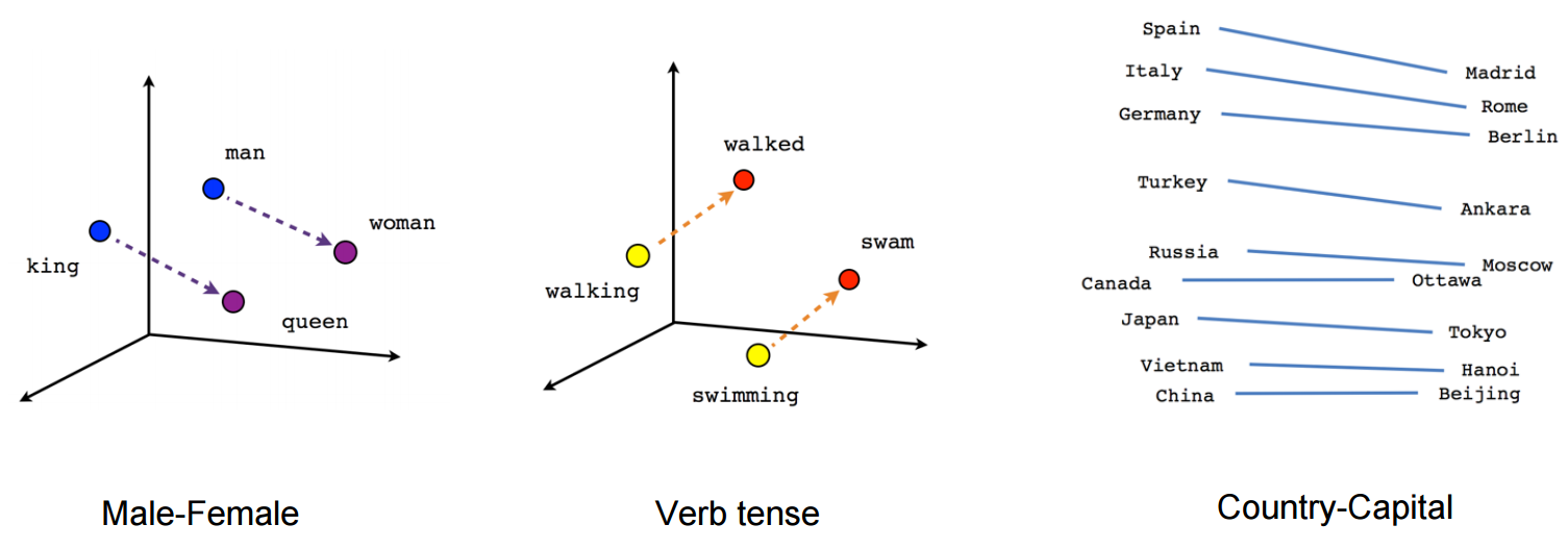
This approach simultaneously learnt how to organize concepts and abstract relations, such as countries capitals, verb tenses, gender-aware words.
Problem with this approach is that it assigned exactly one vector for each word, which is why it is considered as static word embeddings. This is particularly problematic when embedding words with multiple meaning (i.e. polysemous words), such as the word open; it can mean uncovered, honest, or available, depending on the context.
Dynamic (Contextualized) Word Embeddings
Dynamic: Because instead of having a dictionary of word embeddings, where each token in the vocab is stored with its vector representation, a deep neural network is trained and used a word-embedding generator. Most importantly, this word-embedding generator network can be plugged into other deep learning models to be fine-tuned for downstream tasks, in what is commonly known as Transfer Learning.
Contextualized: Because the model is just a network that given a word and a context produces the vector representation of that word for that context.
Sentence Encoders
Bag-of-Words (BOW)
To represent a sentence as a vector, the vectors of the words in that sentence used to be summed or averaged together, in what is called Bag-of-Words (BOW) approach. However, this approach causes the loss of the order information of the word. For example, the sentence "john eats a chicken" and the sentence "a chicken eats john" both would have the same sentence embedding.
Deep Averaging Network (DAN)
One solution to learn how to combine word vectors in a way that maintains the semantic meaning of a sentence is to use a custom neural network designed just to learn how to combine word embeddings in a way that captures the meaning of the sentence.
Universal Sentence Encoder
Is a family of pre-trained sentence encoders by Google, ready to convert a sentence to a vector representation without any additional training, in a way that captures the semantic similarity between sentences.
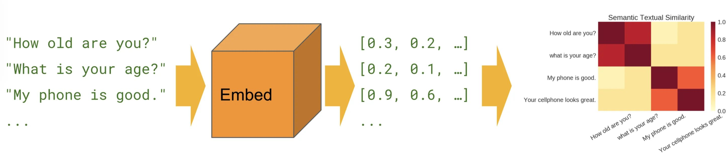
We will be using the pre-trained multilingual model, which works for 16 different languages! It represents sentences using 512-dimensional vectors.
import numpy as np
import tensorflow_hub as hub
import tensorflow_text  # this needs to be imported to set up some stuff in the background
With a single line, we just plug in the url of the pre-trained model and load it.
embed = hub.load("https://tfhub.dev/google/universal-sentence-encoder-multilingual/3")
import re

import pandas as pd
import string

import preprocessor as p
from spacy.lang.en import stop_words as spacy_stopwords  # we use spacy's list of stop words to clean our data

p.set_options(p.OPT.URL, p.OPT.MENTION)  # removes mentions and URLs only
stop_words = spacy_stopwords.STOP_WORDS
punctuations = string.punctuation


def clean(text):
    text = p.clean(text)
    text = re.sub(r'\W+', ' ', text)  # remove non-alphanumeric characters
    # replace numbers with the word 'number'
    text = re.sub(r"\d+", "number", text)
    # don't consider sentenced with less than 3 words (i.e. assumed noise)
    if len(text.strip().split()) < 3:
        return None
    text = text.lower()  # lower case everything

    return text.strip() # remove redundant spaces
df = pd.read_csv("stocktwits (1).csv")
df = df.assign(clean_text=df.message.apply(clean)).dropna()
df
from sklearn.model_selection import train_test_split
import tensorflow as tf
# we split the data into train and test
msg_train, msg_test, y_train, y_test = train_test_split(df.clean_text, df.sentiment)
# we just feed in the list of sentences, and we get the vector representation of each sentence
X_test = embed(msg_test)
X_test.shape
# we don't have enough memory to apply embeddings in one shot,
# so we have to split the data into batches and concatenate them later
splits = np.array_split(msg_train, 5)
l = list()
for split in splits:
    l.append(embed(split))
X_train = tf.concat(l, axis=0)
del l
X_train.shape
We can then use the vector representation of the sentences as features and employ these features in a text classification task, such as classifying a tweet as Bullish or Bearish. Literature suggests that Support Vector Machines (SVM) well with Universal Sentence Encoders. So we will be using that.
SVM Classifier
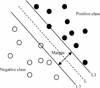
SVM classifiers do not just find a line (or in high dimensions, a hyperplane) that separates the two classes. They try to find the best line that separates them. The objective of SVM classifiers is to maximize the margin between the positive class and the negative class. This margin is defined as the distance between two Support Vectors, hence the name.
from sklearn.svm import SVC
from sklearn.utils.class_weight import compute_class_weight
from sklearn.metrics import classification_report
from sklearn.linear_model import LogisticRegression
Since the data is very imbalanced, we assign higher weights to the lower-represented class
class_weight = compute_class_weight(
    class_weight='balanced', classes=["Bullish","Bearish"], y=y_train
)
class_weight
# initialize the model and assign weights to each class
clf = SVC(class_weight={"Bullish":class_weight[0], "Bearish":class_weight[1]})
# train the model
clf.fit(X_train, y_train)
# use the model to predict the testing instances
y_pred = clf.predict(np.array(X_test))
# generate the classification report
print(classification_report(y_test, y_pred))
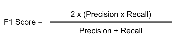
We notice that the model still struggles to detect some of the under-represented samples. We know that Bearish samples are underrepresented by inspecting their support, which refers to how many samples are used in evaluation in this report, and they reflect the same ratio used in the training. In such imbalanced data, accuracy is not a reliable score, as the model can simply classify everything as the dominant class (in this case, Bullish), and get away with a very high accuracy. Instead, we are interested in the f1-score, specifically the macro avg f1-score, which is the average of f1-score for each class.
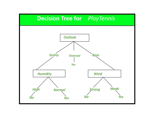
For the sake of experiment, let's also try a Random Forest Classifier. Random Forest, as the name suggests, are basically forests of randomly generated Decision Trees. The concensus of the decision trees in the forest is used to make the final prediction. A decision tree looks like ...
clf = RandomForestClassifier(class_weight={"Bullish":class_weight[0], "Bearish":class_weight[1]})
clf.fit(X_train, y_train)
y_pred = clf.predict(np.array(X_test))
print(classification_report(y_test, y_pred))
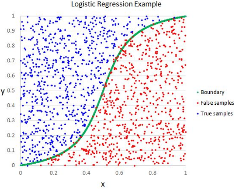
Logisitc Regression is a model that tries to fit an S-shaped curve to the data. The objective of Logisitc Regression is to maximize the likelihood of the probability of the predicted class to match the actual class of a point.
clf = LogisticRegression(class_weight={"Bullish":class_weight[0], "Bearish":class_weight[1]})
clf.fit(X_train, y_train)
y_pred = clf.predict(np.array(X_test))
print(classification_report(y_test, y_pred))
Our findings aggree with the literature that SVM classifiers perform the best with the universal sentence encoders. However, it is worth noting that SVM took almost 9 minutes for the entire experiment to conclude, while Random Forest took just about 40 seconds, and Logistic Regression took only slightly over 2 seconds.
Related Notebooks
- Understanding Word Embeddings Using Spacy Python
- SVM Sklearn In Python
- How to Generate Embeddings from a Server and Index Them Using FAISS with API
- How To Solve Linear Equations Using Sympy In Python
- Crawl Websites Using Python
- Remove An Item From A List In Python Using Clear Pop Remove And Del
- Understanding Logistic Regression Using Python
- TTM Squeeze Stocks Scanner Using Python
- Demystifying Stock Options Vega Using Python