Understanding Standard Deviation With Python
Standard deviation is a way to measure the variation of data. It is also calculated as the square root of the variance, which is used to quantify the same thing. We just take the square root because the way variance is calculated involves squaring some values.
Here is an example question from GRE about standard deviation:
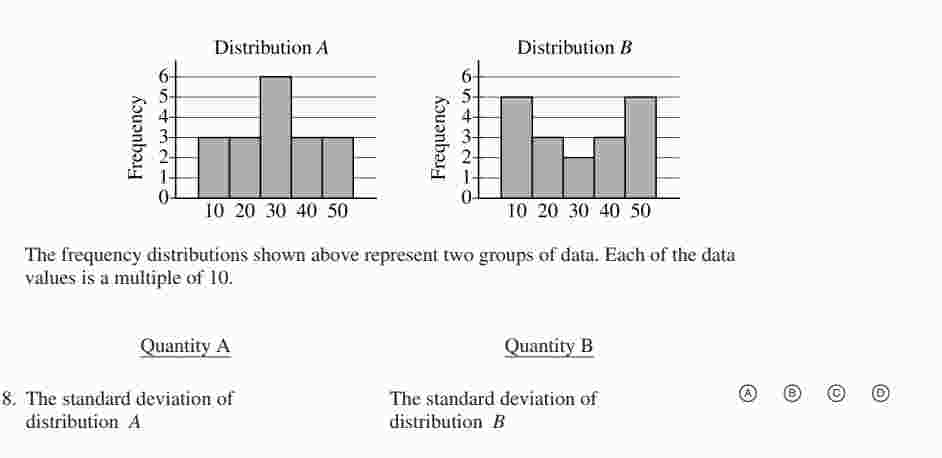
We see that most of the values in group A are around 3. Whereas, values in group B vary a lot. Therefore, the standard deviation of group B is larger than the standard deviation of group A.
import numpy as np

np.mean([60, 110, 105, 100, 85])
Mean (aka average)
Some people claim that there is a difference between the intelligence of men and women. You wanted to explore this claim by getting the IQ values of 5 men and 5 women. Their IQ scores are:
| Men | Women |
|---|---|
| 70 | 60 |
| 90 | 110 |
| 120 | 105 |
| 100 | 100 |
| 80 | 85 |
You can calculate the average IQ for men and women by simply summing up all the IQ scores for each group, and dividing by the group's size. We denote the average (aka mean) with $\mu$ for each data point $x_i$ out of $n$ data points. $$\mu = \frac{1}{n}\sum_{i=1}^n{x_i}$$
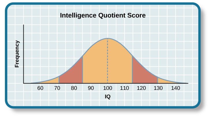
Normal Distributions
In a normal distrubtion, values that appear more often contribute more to the calculation of the average value. In other words, more frequent values are closer to the mean. Conversely, the probability of a value gets higher as the value gets closer to the mean. Wherease, values further away from the mean have less and less probability.
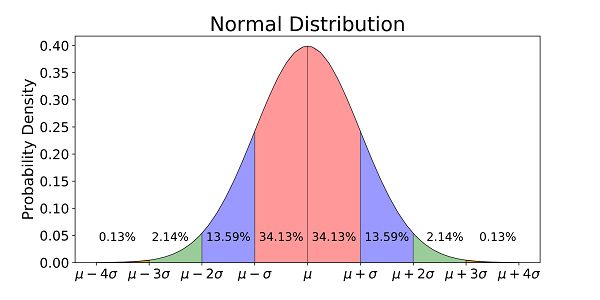
Normal Distribution is a bell-shaped curve that describes the probability or frequency of seeing a range of values. The middle point of the curve is the mean $\mu$, and we quantify the deviation from the mean using standard deviation $\sigma$.
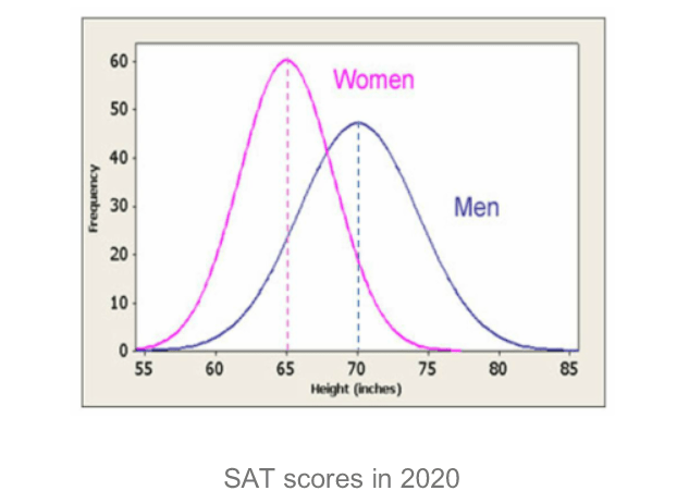
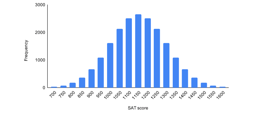
Normal distributions are present in so many contexts in reallife. For example,
Normal distributions can be defined using only the mean $\mu$ and the standard deviation $\sigma$.
Standard Deviation Python
Let's generate a random sample based on a normal distribution and plot the frequency of the values, in what is called histogram.
import matplotlib.pyplot as plt
from scipy.stats import norm
import numpy as np
# generating multiple normal distributions
domain = np.linspace(-2, 2, 1000) # dividing the distance between -2 and 2 into 1000 points

means = [-1, 1, 0]
std_values = [0.1, 0.25, 0.5]

plt.figure(figsize=(16, 9))
for mu, std in zip(means, std_values):
    # pdf stands for Probability Density Function, which is the plot the probabilities of each range of values
    probabilities = norm.pdf(domain, mu, std)
    plt.plot(domain, probabilities, label=f"$\mu={mu}$\n$\sigma={std}$\n")

plt.legend()
plt.xlabel("Value")
plt.ylabel("Probability")
plt.show()
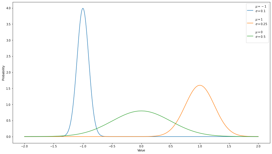
Notice that the larger the standard deviation $\sigma$, the flatter the curve; more values are away from the mean, and vice versa.
Variance & Standard Deviation
We calculate the variance of a set of datapoints by calculating the average of their squared distances from the mean. Variance is the same as standard deviation squared. $$\text{variance}= \sigma^2 = \frac{1}{n}\sum_{i=1}^n{(x_i - \mu)^2}$$ Therefore, $$\sigma =\sqrt{\text{variance}} = \sqrt{\frac{1}{n}\sum_{i=1}^n{(x_i - \mu)^2}}$$
# given a list of values
# we can calculate the mean by dividing the sum of the numbers over the length of the list
def calculate_mean(numbers):
    return sum(numbers)/len(numbers)

# we can then use the mean to calculate the variance
def calculate_variance(numbers):
    mean = calculate_mean(numbers)

    variance = 0
    for number in numbers:
        variance += (mean-number)**2

    return variance / len(numbers)

def calculate_standard_deviation(numbers):
    variance = calculate_variance(numbers)
    return np.sqrt(variance)
Let's test it out!
l = [10, 5, 12, 2, 20, 4.5]
print(f"Mean: {calculate_mean(l)}")
print(f"Variance: {calculate_variance(l)}")
print(f"STD: {calculate_standard_deviation(l)}")
Numpy Standard Deviation
We can do these calculations automatically using NumPy.
array = np.array([10, 5, 12, 2, 20, 4.5])
print(f"Mean:\t{array.mean()}")
print(f"VAR:\t{array.var()}")
print(f"STD:\t{array.std()}")
Standard Deviation Applications
- We use standard deviations to detect outliers in the dataset. If a datapoint is multiple standard-deviations far from the mean, it is very unlikely to occur, so we remove it from the data.
- We use standard deviations to scale values that are normally distributed. So if there are different datasets, each with different ranges (e.g. house prices and number of rooms), we can scale these values to bring them to the same scale by simply dividing the difference between the mean and each value by the standard deviation of that data. $$\tilde{x_g} = \frac{x_g-\mu_g}{\sigma_g}$$ Where $\tilde{x_g}$ is the scaled data point $x$ from the group $g$, and $\sigma_g$ is the standard deviation of values in group $g$.
def scale_values(values):
    std = calculate_standard_deviation(values)
    mean = calculate_mean(values)
    transformed_values = list()
    for value in values:
        transformed_values.append((value-mean)/std)
    return transformed_values
house_prices = [100_000, 500_000, 300_000, 400_000]
rooms_count = [1, 3, 2, 2]
scale_values(house_prices)
scale_values(rooms_count)
And voiala! the transformed values have much closer scale than the original values. Each transformed value is showing how many standard deviations away from the mean is the original value.
# mean and std of house prices
np.mean(rooms_count), np.std(rooms_count)
therefore, a house with 3 rooms is $\frac{1}{\sigma} away from the mean.
This can also be automatically calculated using sklearn
house_prices_array = np.array([house_prices]).T # we transpose it be cause each row should have one value
house_prices_array
rooms_count_array = np.array([rooms_count]).T # we transpose it be cause each row should have one value
rooms_count_array
from sklearn.preprocessing import StandardScaler
scaler=  StandardScaler()
scaler.fit_transform(house_prices_array)
scaler.fit_transform(rooms_count_array)
Related Notebooks
- Understanding Autoencoders With Examples
- Data Cleaning With Python Pdpipe
- With Open Statement in Python
- How To Install Python With Conda
- Regularization Techniques in Linear Regression With Python
- Learn And Code Confusion Matrix With Python
- Merge and Join DataFrames with Pandas in Python
- How To Get Measures Of Spread With Python
- Decision Tree Regression With Hyper Parameter Tuning In Python