Support Vector Machine is one of the classical machine learning algorithm.
It will solve the both Classification and Regression problem statements.
Before going deep down into the algorithm we need to undetstand some basic concepts
(i) Linaer & Non-Linear separable points
(ii) Hyperplane
(iii) Marginal distance
(iv) Support vector
from IPython.display import Image
Image(filename='svm-classification.png',width = 600, height = 300)
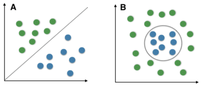
Linear separable points : If you obsereve the above fig A we have 2 class(green,blue) points.By using a line/hyperplane(3D) we can easily separtate these points.These type of points are called as linear separable points
Non-Linear separable points : If you observe the above fig B we have 2 class(green,blue) points we can't separate these points by using line/hyperplane(3D).These type of points are called as Non-Linear separable points.
Image(filename="SVM_hyperplane.png",width = 400, height = 200)
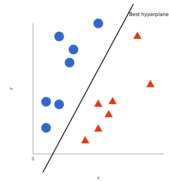
Hyperplane : The line/plane/hyperplane which separates the different class points
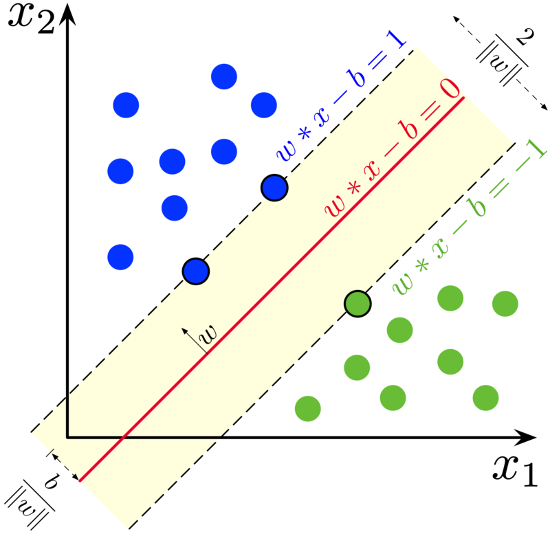
Image(filename="SVM_marginal_distance.png",width = 600, height = 300)
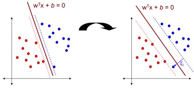
If you observe the above two images the major differnece is the distance between dotted lines. The two dotted lines(blue,red dotted lines) are parallel to the hyperplane. If the distance between these two is large then there is less chance to be misclassification.
In SVM, the distance between these two dotted lines is called Margin.
Image(filename="SVM_support_vectors.png",width = 600, height = 300)
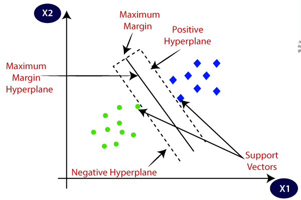
If you observe the above image the data points which passes through the dotted lines(both red,blue lines) are called as support vectors
These support vectors are very helpful to interpret the data point misclassified or not
The maximum distance is called margin
In linear speparable data the higher the marginal distance then our model more generalized model
The Objective is to make higher marginal distance so that we can easily separate the both the classes
Note : For Non-linear separable case svm doesn't give good results. That's why we us SVM Kernals for Non-linear case
SVM : Support Vector Machine is a linear model for classification and regression problems. It can solve linear and non-linear problems and work well for many practical problems. The idea of SVM is simple, The algorithm creates a line or a hyperplane which separates the data into classes.
Objective of SVM is creating maximum marginal distance to build generalized model
Image(filename="svm_hyperplane_equation.png",width = 400, height = 200)
Please checkout more about algorithm here
Image(filename="svm_regularization_lossfunction.png",width = 600, height = 300)
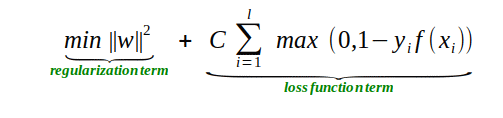
Above equation is the objective function of SVM classification
In the equation we have two terms one is regularization term and another is loss term
In the loss term we have 'C', it's the hyperparameter trade-off is controlled by 'C'
C parameter adds a penalty for each misclassified data point. If c is small, the penalty for misclassified points is low so a decision boundary with a large margin is chosen at the expense of a greater number of misclassifications.
If c is large, SVM tries to minimize the number of misclassified examples due to high penalty which results in a decision boundary with a smaller margin. Penalty is not same for all misclassified examples. It is directly proportional to the distance to decision boundary.
Upto now discussed things works for Linear separable data.
For Non-linear separable data we need to SVM Kernals
Image(filename="SVM_kernels.png",width = 600, height = 300)
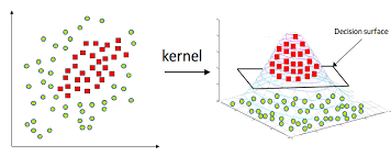
If you observe the above image data is Non-linear separable data. By using mariginal distance technique we can't separate the data points
For this case we use Kernals . Kernals is nothing but similarity(degree closeness) checking.
The working principle of kernal is transforming 2D data points into high dimensonality and then separate those points using plane/hyperplane
Most commonly used keranl function is Radia baisi function(RBF).
Image(filename="SVM_RBF_kernel.png")
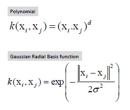
Kernal(RBF) svm objective function
Image(filename="SVM_RBF_objective_function.png")
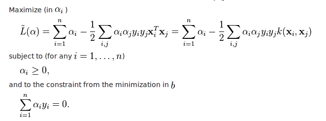
In RBF kernal funtion gamma is the hyperparameter. In Kernal SVM we need to optimize both C,gamma.
Gamma parameter of RBF controls the distance of influence of a single training point. Low values of gamma indicates a large similarity radius which results in more points being grouped together
For high values of gamma, the points need to be very close to each other in order to be considered in the same group (or class)
Note : For a linear kernel, we just need to optimize the c parameter. However, if we want to use an RBF kernel, both c and gamma parameter need to optimized simultaneously. If gamma is large, the effect of c becomes negligible. If gamma is small, c affects the model just like how it affects a linear model.
SVM is also used for regression problems but most of the time SVM is used for classification problems.
I am choosing familar dataset because here my objective is to explain SVM alogrithms and it's hyperparameters.
Linearly Separable Data :
For this purpose, I’m going to use only two features and two classes of the Iris dataset (which contains 4 features and 3 classes). To do so, let’s first have a look at the correlation among features, so that we can pick features and classes which guarantee a linearly-separable data.
# loading Iris data set

import seaborn as sns
iris = sns.load_dataset("iris")
print(iris.head())
y = iris.species
X = iris.drop('species',axis=1)
sns.pairplot(iris, hue="species",palette="bright")
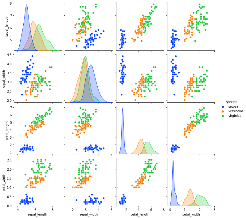
If you observe the above pair plots, petal_length and petal_width features are eaisly separable.
Let us drop sepal_length and sepal_width since we are focusing on petal_length and petal_width for now.
# I am keeping only 2 classes setosa ,versicolor and droppping others

import matplotlib.pyplot as plt

df=iris[(iris['species']!='virginica')]
df=df.drop(['sepal_length','sepal_width'], axis=1)
df.head()
Let us convert categorical values to numerical values first.
# converting class names into numerical forms
# plot between setosa and versicolor

df=df.replace('setosa', 0)
df=df.replace('versicolor', 1)
X=df.iloc[:,0:2]
y=df['species']
plt.scatter(X.iloc[:, 0], X.iloc[:, 1], c=y, s=50, cmap='autumn')
plt.show()
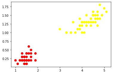
If you observe the above plot we can easily separate these two classes with line.
from sklearn.svm import SVC
model = SVC(kernel='linear')
model.fit(X, y)
Coordianates of support vectors
model.support_vectors_
Visualize the SVM support vectors.
plt.scatter(X.iloc[:, 0], X.iloc[:, 1], c=y, s=50, cmap='autumn')
plt.scatter(model.support_vectors_[:,0],model.support_vectors_[:,1])
plt.show()
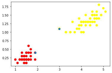
If you observe the above scatter plot, the blue color points are support vectors.
# Now visualizing the mariginal distance and hyperplane
import numpy as np


ax = plt.gca()
plt.scatter(X.iloc[:, 0], X.iloc[:, 1], c=y, s=50, cmap='autumn')
xlim = ax.get_xlim()
ylim = ax.get_ylim()

xx = np.linspace(xlim[0], xlim[1], 30)
yy = np.linspace(ylim[0], ylim[1], 30)
YY, XX = np.meshgrid(yy, xx)
xy = np.vstack([XX.ravel(), YY.ravel()]).T
Z = model.decision_function(xy).reshape(XX.shape)

ax.contour(XX, YY, Z, colors='k', levels=[-1, 0, 1], alpha=0.5,
           linestyles=['--', '-', '--'])

ax.scatter(model.support_vectors_[:, 0], model.support_vectors_[:, 1], s=100,
           linewidth=1, facecolors='none', edgecolors='k')
plt.show()
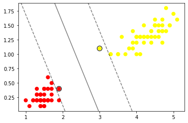
If you observe the above scatter plot we have hyperplane and marginal distance dotted lines.
# data frame
iris.head()
Let us convert Categorical features into numerical features first.
iris['species']=iris['species'].replace('setosa',0)
iris['species']=iris['species'].replace('virginica',1)
iris['species']=iris['species'].replace('versicolor',2)
# dividing  independent and dependent features
X= iris.iloc[:,:-1]
y= iris.iloc[:,-1]
Let us Split the dataframe into train and test data using Sklearn.
from sklearn.model_selection import train_test_split

X_train, X_test, y_train, y_test = train_test_split( X,y,  test_size = 0.30, random_state = 101)
# importing metrics

from sklearn.metrics import classification_report
model = SVC()
model.fit(X_train, y_train)

# model prediction results on test data

predictions = model.predict(X_test)
print(classification_report(y_test, predictions))
If you observe the classification report without hyperparameter tuning, we are getting accuracy 98% and f1 score values for Class 0 is 100% , for class 1 is 96% and for class 2 is 97%.
we are taking small data set so we are getting good values but what about complex data sets . When we have complex data sets, we don't get good metric values until we tune the hyperparameters of SVM algorithm.
In the SVM 'C' & gamma are hyperparameters . we can find best hyperparameters using GridSearchCV and RandomizedSearchCV.
GridsearchCV checks the all possibilites in the given hyperparameter values space.
%%capture
from sklearn.model_selection import GridSearchCV
from sklearn.svm import SVC

# defining parameter range
param_grid = {'C': [0.1, 1, 10, 100, 1000],
              'gamma': [1, 0.1, 0.01, 0.001, 0.0001],
              'kernel': ['rbf','linear']}

grid = GridSearchCV(SVC(), param_grid, refit = True, verbose = 3)

# fitting the model for grid search
grid.fit(X_train, y_train)
# best parameters by GridsearchCV
print(grid.best_params_)
# best estimatior
print(grid.best_estimator_)
Now let us predict the test values using the hyper parameters from GridsearchCV.
grid_predictions = grid.predict(X_test)
print(classification_report(y_test, grid_predictions))
If you observe the above classification_report accuracy is 100% and f1 score for all three classes is also 100% . This is very small data set that's the reason we are getting the perfect results.
Bottom line is that tuning Hypertuning parameters improve the model substantially.
For this example, I am creating my own sample of Non linear separable dataset as shown below.
# creating non linear dataset samples

from sklearn.datasets import make_circles

X,y = make_circles(n_samples=100, factor=.1, noise=.1)
Let us visualize our non linear data first using a scatter plot.
import matplotlib.pyplot as plt
plt.scatter(X[:, 0], X[:, 1], c=y, s=50, cmap='autumn')
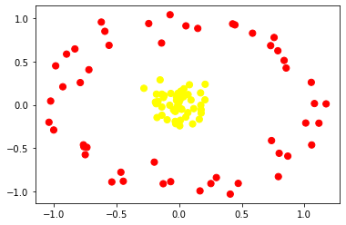
If you observe the above scatter plot we can't separate two classes with line.
To solve above problem statement we are using SVM kernal
SVM kernal: transform the points into higer dimensions and then we can easily separate these points using a hyperplane.
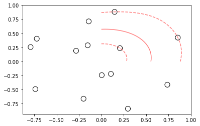
# trying linear svm on non-linear separable data

model=SVC(kernel='linear').fit(X, y)

ax = plt.gca()
xlim = ax.get_xlim()
ylim = ax.get_ylim()
# create grid to evaluate model
xx = np.linspace(xlim[0], xlim[1], 30)
yy = np.linspace(ylim[0], ylim[1], 30)
YY, XX = np.meshgrid(yy, xx)
xy = np.vstack([XX.ravel(), YY.ravel()]).T
Z = model.decision_function(xy).reshape(XX.shape)
# plot decision boundary and margins
ax.contour(XX, YY, Z, colors='r', levels=[-1, 0, 1], alpha=0.5,
           linestyles=['--', '-', '--'])
# plot support vectors
ax.scatter(model.support_vectors_[:, 0], model.support_vectors_[:, 1], s=100,
           linewidth=1, facecolors='none', edgecolors='k')
plt.show()
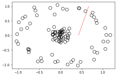
If you observe the above scatter plot, inner circular points (yellow color points in the previous scatter plot) and outer circlar points(red color circular points in the previous scatter plot) are not separated as efficently as we saw in the linear separable data set example above.
Ok, Let us visualize our data in 3D space using numpy and mplot3d.
#  converting non linear separable data from 2D to 3D


from mpl_toolkits import mplot3d
#setting the 3rd dimension with RBF centered on the middle clump
r = np.exp(-(X ** 2).sum(1))
ax = plt.subplot(projection='3d')
ax.scatter3D(X[:, 0], X[:, 1], r, c=y, s=50, cmap='autumn')
ax.set_xlabel('x')
ax.set_ylabel('y')
ax.set_zlabel('r')
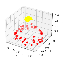
If you observe, in the above scatter plot, both the red and yellow color points are easily separable using plane/hyperplane.
we don't need to convert these non linear separable data into 3 dim because SVM kernal take cares of that.
# Fiiting the train data SVM kernal . For nan linear separable data I am using RBF kernal

model=SVC(kernel='rbf').fit(X, y)
# visualizing the hyperplane and marginal distance in non linear separable data

ax = plt.gca()
xlim = ax.get_xlim()
ylim = ax.get_ylim()
# create grid to evaluate model
xx = np.linspace(xlim[0], xlim[1], 30)
yy = np.linspace(ylim[0], ylim[1], 30)
YY, XX = np.meshgrid(yy, xx)
xy = np.vstack([XX.ravel(), YY.ravel()]).T
Z = model.decision_function(xy).reshape(XX.shape)
# plot decision boundary and margins
ax.contour(XX, YY, Z, colors='r', levels=[-1, 0, 1], alpha=0.5,
           linestyles=['--', '-', '--'])
# plot support vectors
ax.scatter(model.support_vectors_[:, 0], model.support_vectors_[:, 1], s=100,
           linewidth=1, facecolors='None', edgecolors='k')
plt.show()
Image(filename="svm_nonlinear_decision_boundary.png",width = 400, height = 200)
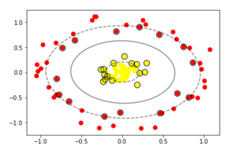
If you observe the above scatter plot, we have 1 hyperplane between inner and outer circular points.
Also have higher marginal distance
- SVM is Simple and effective.
- It can solve linear and non linear problems.
- Try for linear separable data - linear kernel and for Non-linear separable data - rbf kernel(most commonly used kernel).
- Try tuning Hyperparameters using range: 0.0001 < gamma < 10 and 0.1 < c < 100
- No need to worry about feature engineering or feature transformtion because SVM can take care of it by Kernels.
- SVM is less impacted by outliers.
- Interpretability is not easy in SVM because interpreting kernels is very hard.
- SVM is not for doing feature selection.
- For Higher dimensional data, SVM works very well if we choose an appropriate kernal for classification.
Related Notebooks
- Polynomial Interpolation Using Python Pandas Numpy And Sklearn
- Word Embeddings Transformers In SVM Classifier Using Python
- Append In Python
- Dictionaries In Python
- Activation Functions In Python
- Set Operations In Python
- Pivot Tables In Python Pandas
- Strftime and Strptime In Python
- Object Oriented Programming In Python