Summarising, Aggregating, and Grouping data in Python Pandas

In this post, I will talk about summarizing techniques that can be used to compile and understand the data. I will use Python library Pandas to summarize, group and aggregate the data in different ways.

I will be using college.csv data which has details about university admissions.

Lets start with importing pandas library and read_csv to read the csv file

In [1]:
import pandas as pd
In [2]:
df = pd.read_csv('College.csv')

Lets understand the data first. We can pass in an argument "a number" to head function. I will print out the first two rows of the data using pandas head function.

In [3]:
df.head(2)
Out[3]:
Unnamed: 0 Private Apps Accept Enroll Top10perc Top25perc F.Undergrad P.Undergrad Outstate Room.Board Books Personal PhD Terminal S.F.Ratio perc.alumni Expend Grad.Rate
0 Abilene Christian University Yes 1660 1232 721 23 52 2885 537 7440 3300 450 2200 70 78 18.1 12 7041 60
1 Adelphi University Yes 2186 1924 512 16 29 2683 1227 12280 6450 750 1500 29 30 12.2 16 10527 56

Looking at the data, we have both textual, categorical and numerical data. Lets first fix the university column name which is "Unnamed:0"

In [4]:
df.rename(columns={'Unnamed: 0':'univ_name'},inplace=True)
In [5]:
df.head(1)
Out[5]:
univ_name Private Apps Accept Enroll Top10perc Top25perc F.Undergrad P.Undergrad Outstate Room.Board Books Personal PhD Terminal S.F.Ratio perc.alumni Expend Grad.Rate
0 Abilene Christian University Yes 1660 1232 721 23 52 2885 537 7440 3300 450 2200 70 78 18.1 12 7041 60

OK, now we have fixed the column name, lets start with tutorial now. I will talk about how to summarize first.

How to summarize the data using Python Pandas

Easiest way is to use describe function of Python Pandas. Lets first use it and see and what happens.

In [6]:
df.describe()
Out[6]:
Apps Accept Enroll Top10perc Top25perc F.Undergrad P.Undergrad Outstate Room.Board Books Personal PhD Terminal S.F.Ratio perc.alumni Expend Grad.Rate
count 777.000000 777.000000 777.000000 777.000000 777.000000 777.000000 777.000000 777.000000 777.000000 777.000000 777.000000 777.000000 777.000000 777.000000 777.000000 777.000000 777.00000
mean 3001.638353 2018.804376 779.972973 27.558559 55.796654 3699.907336 855.298584 10440.669241 4357.526384 549.380952 1340.642214 72.660232 79.702703 14.089704 22.743887 9660.171171 65.46332
std 3870.201484 2451.113971 929.176190 17.640364 19.804778 4850.420531 1522.431887 4023.016484 1096.696416 165.105360 677.071454 16.328155 14.722359 3.958349 12.391801 5221.768440 17.17771
min 81.000000 72.000000 35.000000 1.000000 9.000000 139.000000 1.000000 2340.000000 1780.000000 96.000000 250.000000 8.000000 24.000000 2.500000 0.000000 3186.000000 10.00000
25% 776.000000 604.000000 242.000000 15.000000 41.000000 992.000000 95.000000 7320.000000 3597.000000 470.000000 850.000000 62.000000 71.000000 11.500000 13.000000 6751.000000 53.00000
50% 1558.000000 1110.000000 434.000000 23.000000 54.000000 1707.000000 353.000000 9990.000000 4200.000000 500.000000 1200.000000 75.000000 82.000000 13.600000 21.000000 8377.000000 65.00000
75% 3624.000000 2424.000000 902.000000 35.000000 69.000000 4005.000000 967.000000 12925.000000 5050.000000 600.000000 1700.000000 85.000000 92.000000 16.500000 31.000000 10830.000000 78.00000
max 48094.000000 26330.000000 6392.000000 96.000000 100.000000 31643.000000 21836.000000 21700.000000 8124.000000 2340.000000 6800.000000 103.000000 100.000000 39.800000 64.000000 56233.000000 118.00000

As we see above, All the numberical columns have been statistically summarized by the describe() function. For every column, Pandas has given us a nice summary count, mean, standard deviation (std), min, max, 25 percentile, 50 percentile and 75 percentile. This is good. We can also call a plot method on the describe() method to see the plots of different columns. Lets try that and see what happens.

For that we need to first execute %matplotlib inline so that we can see the plot.

In [7]:
%matplotlib inline
df.describe().plot()
Out[7]:
<matplotlib.axes._subplots.AxesSubplot at 0x7f74f9ab4cd0>

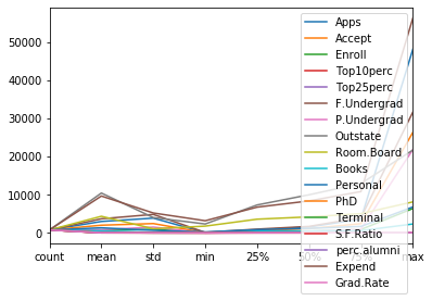
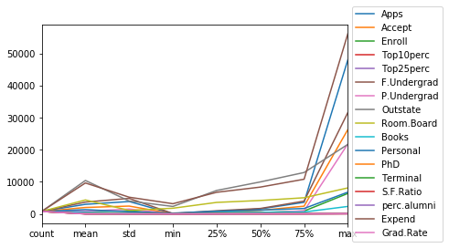
The labels are not aligned properly. Lets fix that quickly using the legend. I wouldn't go in detail about matplotlib and its usage that in itself required a multipart series.

In [8]:
df.describe().plot().legend(loc='center left', bbox_to_anchor=(1, 0.5))
Out[8]:
<matplotlib.legend.Legend at 0x7f74f9a8c710>

Lets continue with our summarize discussion.

We can apply max, min, sum, average, count functions directly on the dataframe for each column. Lets try these methods on Apps column.

In [9]:
df['Apps'].sum()
Out[9]:
2332273
In [10]:
df['Apps'].count()
Out[10]:
777
In [11]:
df['Apps'].max()
Out[11]:
48094
In [13]:
df['Apps'].min()
Out[13]:
81
In [16]:
df['Apps'].mean()
Out[16]:
3001.6383526383524

We can also apply all these methods in one command using Pandas apply method. Lets try to calculate all the above metrics using the apply method in one command.

In [26]:
df['Apps'].apply({'sum':sum,'min':min,'max':max,'count':count,'mean':mean})
---------------------------------------------------------------------------
NameError                                 Traceback (most recent call last)
<ipython-input-26-44af3e04c98d> in <module>
----> 1 df['Apps'].apply({'sum':sum,'min':min,'max':max,'count':count,'mean':mean})

NameError: name 'count' is not defined

Ok, we got the error that count is not defined. count is not vectorized method, therefore we can't use with apply method. However we can use len method of Python.

In [27]:
df['Apps'].apply({'sum':sum,'min':min,'max':max,'count':len,'mean':mean})
---------------------------------------------------------------------------
NameError                                 Traceback (most recent call last)
<ipython-input-27-743e2f3746e4> in <module>
----> 1 df['Apps'].apply({'sum':sum,'min':min,'max':max,'count':len,'mean':mean})

NameError: name 'mean' is not defined

Ok, len has worked but not we got the error that mean is not defined. For that we will have to use method from the numpy library. Numpy is great library for matix calculations.

In [28]:
import numpy as np
In [30]:
df['Apps'].apply({'sum':sum,'min':min,'max':max,'count':len,'mean':np.mean})
Out[30]:
sum      2.332273e+06
min      8.100000e+01
max      4.809400e+04
count    7.770000e+02
mean     3.001638e+03
Name: Apps, dtype: float64

How to aggregate data using Python Pandas aggregate() method

Please checkout below example to see the syntax of Pandas aggregate() method.

In [35]:
df['Apps'].aggregate({'sum':sum,'min':min,'max':max,'count':len,'mean':np.mean})
Out[35]:
sum      2.332273e+06
min      8.100000e+01
max      4.809400e+04
count    7.770000e+02
mean     3.001638e+03
Name: Apps, dtype: float64

Lets try aggregate on all the columns

In [55]:
df.aggregate({sum,min,max,len,np.mean})
Out[55]:
Apps Accept Enroll Top10perc Top25perc F.Undergrad P.Undergrad Outstate Room.Board Books Personal PhD Terminal S.F.Ratio perc.alumni Expend Grad.Rate
mean 3.001638e+03 2.018804e+03 779.972973 27.558559 55.796654 3.699907e+03 855.298584 1.044067e+04 4.357526e+03 549.380952 1.340642e+03 72.660232 79.702703 14.089704 22.743887 9.660171e+03 65.46332
sum 2.332273e+06 1.568611e+06 606039.000000 21413.000000 43354.000000 2.874828e+06 664567.000000 8.112400e+06 3.385798e+06 426869.000000 1.041679e+06 56457.000000 61929.000000 10947.700000 17672.000000 7.505953e+06 50865.00000
len 7.770000e+02 7.770000e+02 777.000000 777.000000 777.000000 7.770000e+02 777.000000 7.770000e+02 7.770000e+02 777.000000 7.770000e+02 777.000000 777.000000 777.000000 777.000000 7.770000e+02 777.00000
min 8.100000e+01 7.200000e+01 35.000000 1.000000 9.000000 1.390000e+02 1.000000 2.340000e+03 1.780000e+03 96.000000 2.500000e+02 8.000000 24.000000 2.500000 0.000000 3.186000e+03 10.00000
max 4.809400e+04 2.633000e+04 6392.000000 96.000000 100.000000 3.164300e+04 21836.000000 2.170000e+04 8.124000e+03 2340.000000 6.800000e+03 103.000000 100.000000 39.800000 64.000000 5.623300e+04 118.00000

Note one difference is that we can't rename the metrics. Although we can rename the names separately. One other thing to notice here is that Aggregate method skipped automatically the textual columns univ_name and Private and only calculated metrics for numerical columns. Although you would see metrics on all the columns if you run following command.

In [56]:
df.aggregate(['sum','min'])
Out[56]:
univ_name Private Apps Accept Enroll Top10perc Top25perc F.Undergrad P.Undergrad Outstate Room.Board Books Personal PhD Terminal S.F.Ratio perc.alumni Expend Grad.Rate
sum Abilene Christian UniversityAdelphi University... YesYesYesYesYesYesYesYesYesYesYesYesYesYesYesY... 2332273 1568611 606039 21413 43354 2874828 664567 8112400 3385798 426869 1041679 56457 61929 10947.7 17672 7505953 50865
min Abilene Christian University No 81 72 35 1 9 139 1 2340 1780 96 250 8 24 2.5 0 3186 10

The output shown above is not meaningful since 'max' of column univ_name and 'Private' dont make any sense. If we use above method, we will have to explictly mentioned for which columns we want to calculate metrics.

In [58]:
df.aggregate({'Apps':['sum','min'],'Accept':'min'})
Out[58]:
Apps Accept
min 81 72.0
sum 2332273 NaN

As we shown above, this way we get more control, we have applied sum and min on Apps method but only applied min on Accept column. If we want to apply same functions to selected columns then do following...

In [59]:
df[['Apps','Accept']].aggregate(['sum','min'])
Out[59]:
Apps Accept
sum 2332273 1568611
min 81 72

Aggregate is very powerful command. We can do much more than what I described above. Lets look at one more scenario. Lets say we want to calculate for the univerisities which are private and non private what is maximum value for each column.

To do that, lets just take out the column 'univ_name', because max of univ_name doesnt make any sense. To group by 'Private' column, we would use Pandas groupby method. groupby will group our entire data set by the unique private entries. In our data set we have only two unique values of 'Private' field 'Yes' and 'No'.

In [100]:
df.loc[:, df.columns != 'univ_name'].groupby('Private').aggregate(max)
Out[100]:
Apps Accept Enroll Top10perc Top25perc F.Undergrad P.Undergrad Outstate Room.Board Books Personal PhD Terminal S.F.Ratio perc.alumni Expend Grad.Rate
Private
No 48094 26330 6392 95 100 31643 21836 15732 6540 1125 4288 103 100 28.8 48 16527 100
Yes 20192 13007 4615 96 100 27378 10221 21700 8124 2340 6800 100 100 39.8 64 56233 118

As we see above, we got maximum value for each column. We can also apply multiple methods to see other metrics too.

In [105]:
df.loc[:, df.columns != 'univ_name'].groupby('Private').aggregate(['max','mean','min'])
Out[105]:
Apps Accept Enroll Top10perc ... S.F.Ratio perc.alumni Expend Grad.Rate
max mean min max mean min max mean min max ... min max mean min max mean min max mean min
Private
No 48094 5729.919811 233 26330 3919.287736 233 6392 1640.872642 153 95 ... 6.7 48 14.358491 0 16527 7458.316038 3605 100 56.042453 10
Yes 20192 1977.929204 81 13007 1305.702655 72 4615 456.945133 35 96 ... 2.5 64 25.890265 2 56233 10486.353982 3186 118 68.998230 15

2 rows × 51 columns

In the above output, we wee max,mean and min for each column for both Private vs non Private Universities.

Wrap Up!

In the above examples, I have just scractched the surface. There is a lot more we can do by combining aggregate and groupby methods of Pandas.