Regularization Techniques in Linear Regression With Python

What is Linear Regression

Linear Regression is the process of fitting a line that best describes a set of data points.

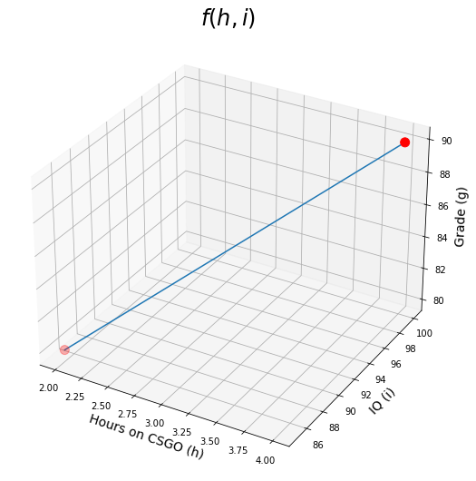
Let's say you are trying to predict the Grade $g$ of students, based on how many hours $h$ they spend playing CSGO, and their IQ scores $i$. So you collected the data for a couple of students as follows:

Hours on CSGO (h)	IQ (i)	Grade (g)
2	85	80
4	100	90

You then lay out this data as a system of equations such as: $$f(h,i) = h.\theta_1 + i.\theta_2=g$$ where $\theta_1$ and $\theta_2$ are what you are trying to learn to have a predictive model. So based on our data, now we have: $$2 \theta_1 + 85 \theta_2=80$$ and $$ 4 \theta_1 + 100 \theta_2=90$$ We can then easily calculate $\theta_1=-2.5$ and $\theta_2=1$.

So now we can plot $f(h,i)=-2.5h+i$

import warnings
warnings.filterwarnings('ignore')
import matplotlib.pyplot as plt
import numpy as np

def grade(h, i):
    return -2.5 * h + i

from mpl_toolkits.mplot3d import Axes3D
fig = plt.figure(figsize=(16,9))
ax = fig.add_subplot(111, projection='3d')
h = np.array([2, 4]) # hours on CSGO from 0 to 10
i = np.array([85, 100]) # IQ from 70 to 130
grades = grade(h, i)
ax.plot(h, i, grades)

ax.scatter([2, 4],[85,100], [80, 90], s=100, c='red') # plotting our sample points

ax.set_xlabel("Hours on CSGO (h)", fontsize=14)
ax.set_ylabel("IQ (i)", fontsize=14)
ax.set_zlabel("Grade (g)", fontsize=14)
plt.title(r"$f(h,i)$", fontsize=24)
plt.show()

What we did so far can be represented with matrix operations. We refer to features or predictors as capital $X$, because there are more than one dimensions usually (for example hours on CSGO is one dimension, and IQ is another). We refer to the target variable (in this case the grades of the students) as small $y$ because target variable is usually one dimension (in our example it is grade). So, in matrix format, that would be: $$X\theta=y$$ THIS EQUATION IS THE NUTSHELL OF SUPERVISED MACHINE LEARNING

Let's expand this matrix-format equation and generalize it.

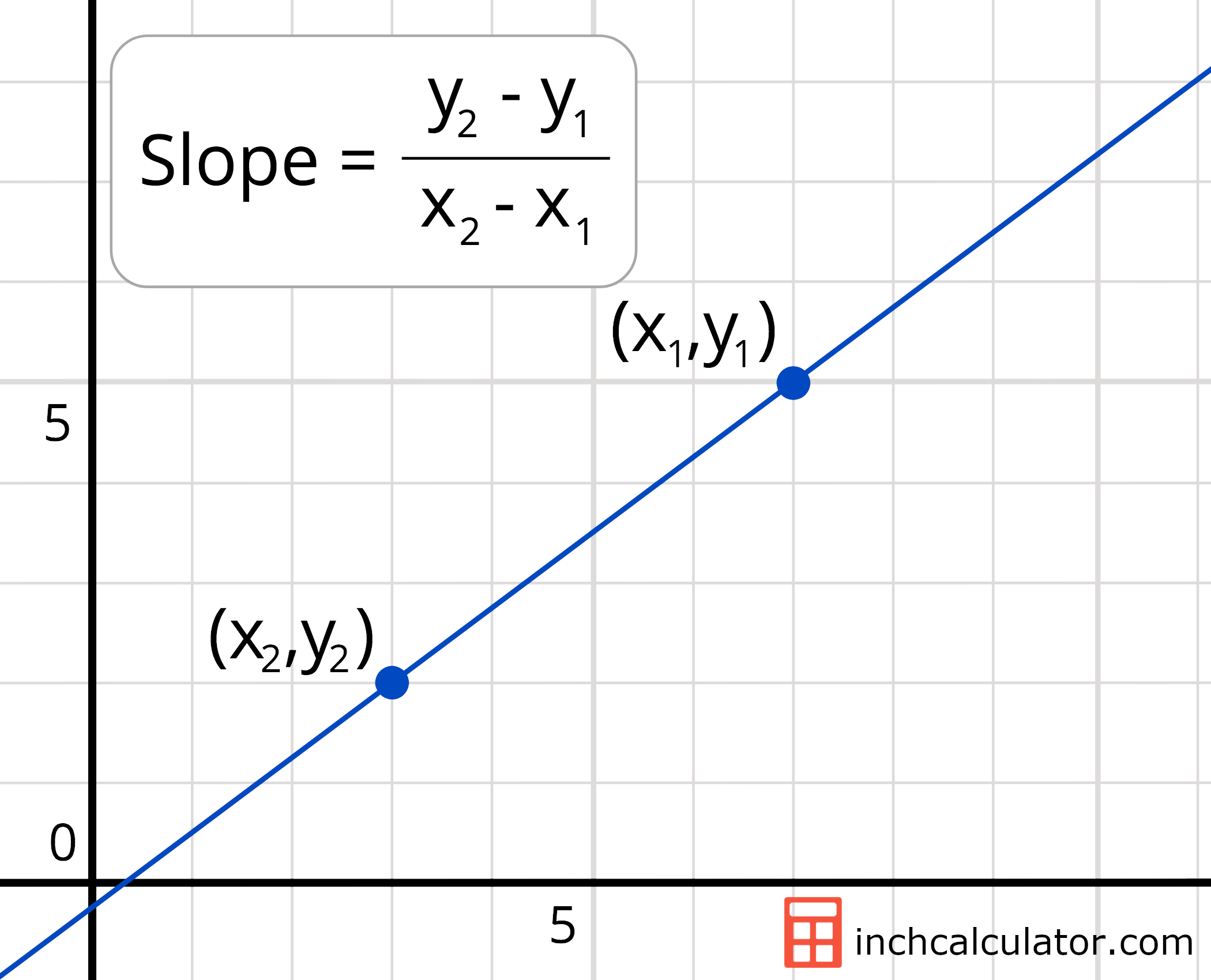
Do we need to draw a line? using:

Two points.
Intercept and slope.

We don't typically have just two points as our data have ton of points and not all of them are on the same line. We are just trying to approximate a line that captures the trend of the data.

Intercept: what y is when x is 0
Slope: how much does y change when x changes

from IPython.display import Image
Image(filename="slope-equation.png",width = 300, height = 100)

As we said earlier, we don't just have one predictor (small $x$), we have many predictors (aka features). In the previous example, we had two variables $x_1$ (hours spent on CSGO) and $x_2$ (the studet's IQ). But we can have more, many many more variables. In other words, $y$ is the linaer combination of all predictors $x_i$ $$y\approx f(x_1, x_2, x_3, ..., x_k) = \beta_0 + \beta_1 x_1 + \beta_2 x_2 + \beta_3 x_3 + ... + \beta_n x_k$$ Where $\beta_0$ is the intercept, and the remaining $\beta$s are the $k$ coefficients of our linear regression model, one for each of the $k$ predictors (aka features).

When we have hundreds of thousands of points, there does not exist a line that can pass through them all. This is where we use line-fitting.

We start by setting the $\theta$ values randomly.
We use the current value of $\theta$ to get the predictions.
We calculate the error by taking the mean of all the squared differenes between the predictions and labels (also called mean squared error MSE) $$MSE=\frac{1}{n}\sum^n_{i=1}{(y_i-\hat{y_i})^2}$$ where $n$ is the number of data points, $y_i$ is one label, and $\hat{y_i}$ is the prediction for that label.
We use the error calculated to update $\theta$ and repeat from 2 to 3 until $\theta$ stops changing.

Linear Regression Using Python Sklearn

Data: Boston housing prices dataset

We will use Boston house prices data set. A typical dataset for regression models.

from sklearn.datasets import load_boston
# loading the data
X, y= load_boston(return_X_y=True) # we want both features matrix X, and labels vector y
X.shape # the dataset has 506 houses with 13 features (or predictors) for a house price in boston

(506, 13)

To use any predictive model in sklearn, we need exactly three steps:

Initialize the model by just calling its name.
Fitting (or training) the model to learn the parameters (In case of Linear Regression these parameters are the intercept and the $\beta$ coefficients.
Use the model for predictons!

import warnings
warnings.filterwarnings('ignore')
from sklearn.linear_model import LinearRegression
# Initialize the model
lr = LinearRegression()
# training the model
# we pass in the features as well as the labels we want to map to (remember the CGSO and IQ = GPA example?)
lr.fit(X, y)
# we can now use the model for predictions! We will just give the same predictors
predictions = lr.predict(X)

Well there are 13 features, meaning the data has 13 dimensions, so we can't visualize them as we did with the CSGO+IQ=GPA example.

But let's see the coefficients of the model, and the intercept too!

# here are the coefficients
lr.coef_

array([-1.08011358e-01,  4.64204584e-02,  2.05586264e-02,  2.68673382e+00,
       -1.77666112e+01,  3.80986521e+00,  6.92224640e-04, -1.47556685e+00,
        3.06049479e-01, -1.23345939e-02, -9.52747232e-01,  9.31168327e-03,
       -5.24758378e-01])

Let us check the Linear Regression intercept.

# the intercept
lr.intercept_

36.459488385089855

The coefficients simultaneously reflect the importance of each feature in predicting the target (which is the house price in this case), but ONLY IF the features are all on the same scale. Say you can only spend 3 to 10 hours on CSGO daily, but IQ values of a student can range from 80 to 110 for example. Predicting the GPA as a linear combination of these two predictors has to give a relatively bigger coefficient to CSGO than IQ, for example, 0.5 for CSGO daily hours of 4 and 0.01 for IQ of 100 will give a nice GPA of 2.1. That's why we sometimes need to scale the features to have all of them range from 0 to 1. Stay tuned!

Linear Regression Loss Function

There are different ways of evaluating the errors. For example, if you predicted that a student's GPA is 3.0, but the student actual GPA is 1.0, the difference between the actual and predicted GPAs is $1.0 - 3.0 = -2.0$. However, there can't be a negative distance, can it be? So what can we do?

Well, you can either take the absolute difference, which is just $2.0$. Alternatively, you can take the squared difference , which is $2.0^2 = 4.0$. If you can't decide which one to use, you can add them together, it is not the end of the world, so it will be $1.0+4.0 = 5.0$. Well, each of these distance calculation techniques (aka distance metrics) result in a differently behaving linear regression model. To escape the ambiguity about the distance between the actual and the predicted value, we use the term residual, which refers to the error, regardless of how it is calculated. So let's put all residual calculation techinques in a table for you, with their formal names and formulas.

Distance Metric	Formal Name	Nickname	Formula
Absolute	Lasso	L1	\|$d$\|
Squared	Ridge	L2	$d^2$
Both	Elastic Net	EN	\|$d$\| + $d^2$

The function we want to normalize when we are fitting a linear regression model is called the loss function, which is the sum of all the squared residuals on the training data, formally called Residual Sum of Squares (RSS): $$RSS = \sum_{i=1}^n{\bigg(y_i-\beta_0-\sum_{j=1}^k{\beta_jx_{ij}}\bigg)^2}$$ Notice the similarity between this equation and the MSE equation defined above. MSE is used to evaluate the performance of the model at the end, and it doesn't not depend on how $\hat{y_i}$ (i.e. the predicted value) is calculated. Whereas, RSS, uses the SS (Sum of Squares) to calculate the residual of all data points in training time.

Regularization

What: Regularization is used to constraint (or regularize) the estimated coefficients towards 0. This protects the model from learning exceissively that can easily result overfit the training data. Even though we are aiming to fit a line, having a combination of many features can be quite complex, it is not exactly a line, it is the k-dimensional version of a line (e.g. k is 13 for our model on the Boston dataset)! Just to approximate the meaning on a visualizable number of dimensions...

Image(filename="regularization.png")

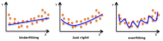
So in other words

Regularization is used to prevent overfitting

BUT

too much regularization can result in underfitting.

We introduce this regularization to our loss function, the RSS, by simply adding all the (absolute, squared, or both) coefficients together. Yes, absolute, squared, or both, this is where we use Lasso, Ridge, or ElasticNet regressions respectively :)

So our new loss function(s) would be:

$\text{Lasso} = RSS + \lambda \sum_{j=1}^k {|\beta_j|}$ $\text{Ridge} = RSS + \lambda \sum_{j=1}^k {\beta_j^2}$ $\text{ElasticNet} = RSS + \lambda \sum_{j=1}^k {(|\beta_j| + \beta_j^2)}$

This $\lambda$ is a constant we use to assign the strength of our regularization. You see if $\lambda=0$ , we end up with good ol' linear regression with just RSS in the loss function. And if $\lambda=\inf$ the regularization term would dwarf RSS, which in turn, because we are trying to minimize the loss function, all coefficients are going to be zero, to counter attack this huge $\lambda$ ., resuling in underfitting.

Scaling

But hold on! We said if the features are not on the same scale, also coefficients are not going to be on the same scale, would that confuse the regularization. Yes it would :( So we need to normalize all the data to be on the same scale. The formula used to do this is for each feature $j$ for a data point $x_i$ from a total of $n$ data points:

$$\tilde{x_{ij}} = \frac{x_{ij}}{\sqrt{\frac{1}{2}\sum_{i=1}^{n}{(x_{ij}-\bar{x_j})^2}}}$$

Where $\bar{x_j}$ is the mean value for that feature over all data points.

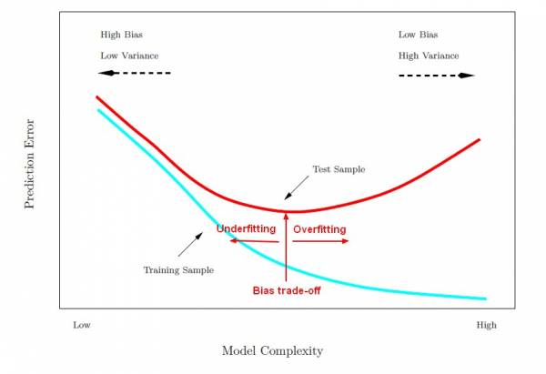
Evaluation

If we can't visualize the data, how are we going to evaluate whether or not the model has overfitted or underfitted?

If it overfitted, that means it would get a very low residual error on the training set, but it might fail miserably on new data. So we split the data into training and testing splits.

Image(filename="model_complexity_error_training_test.jpg")

from sklearn.model_selection import train_test_split

# we set aside 20% of the data for testing, and use the remaining 80% for training
X_train, X_test, y_train, y_test = train_test_split(X, y, test_size=0.2)

Experiment

Now we can see the performance of the model with different regularization strengths, and analyze the difference between each type of regularization.

from sklearn.linear_model import ElasticNet, Lasso, Ridge
from sklearn.metrics import mean_squared_error  # we will use MSE for evaluation
import matplotlib.pyplot as plt

def plot_errors(lambdas, train_errors, test_errors, title):
    plt.figure(figsize=(16, 9))
    plt.plot(lambdas, train_errors, label="train")
    plt.plot(lambdas, test_errors, label="test")
    plt.xlabel("$\\lambda$", fontsize=14)
    plt.ylabel("MSE", fontsize=14)
    plt.title(title, fontsize=20)
    plt.legend(fontsize=14)
    plt.show()

def evaluate_model(Model, lambdas):
    training_errors = [] # we will store the error on the training set, for using each different lambda
    testing_errors = [] # and the error on the testing set
    for l in lambdas:
        # in sklearn, they refer to lambda as alpha, the name is different in different literature
        # Model will be either Lasso, Ridge or ElasticNet
        model = Model(alpha=l, max_iter=1000) # we allow max number of iterations until the model converges
        model.fit(X_train, y_train)

        training_predictions = model.predict(X_train)
        training_mse = mean_squared_error(y_train, training_predictions)
        training_errors.append(training_mse)

        testing_predictions = model.predict(X_test)
        testing_mse = mean_squared_error(y_test, testing_predictions)
        testing_errors.append(testing_mse)
    return training_errors, testing_errors

Lasso L1 Regularization

$$\text{Lasso} = RSS + \lambda \sum_{j=1}^k {|\beta_j|}$$

import warnings
warnings.filterwarnings('ignore')
# let's generate different values for lambda from 0 (no-regularization) and (10 too much regularization)
lambdas = np.arange(0, 10, step=0.1)

lasso_train, lasso_test = evaluate_model(Lasso, lambdas)
plot_errors(lambdas, lasso_train, lasso_test, "Lasso")

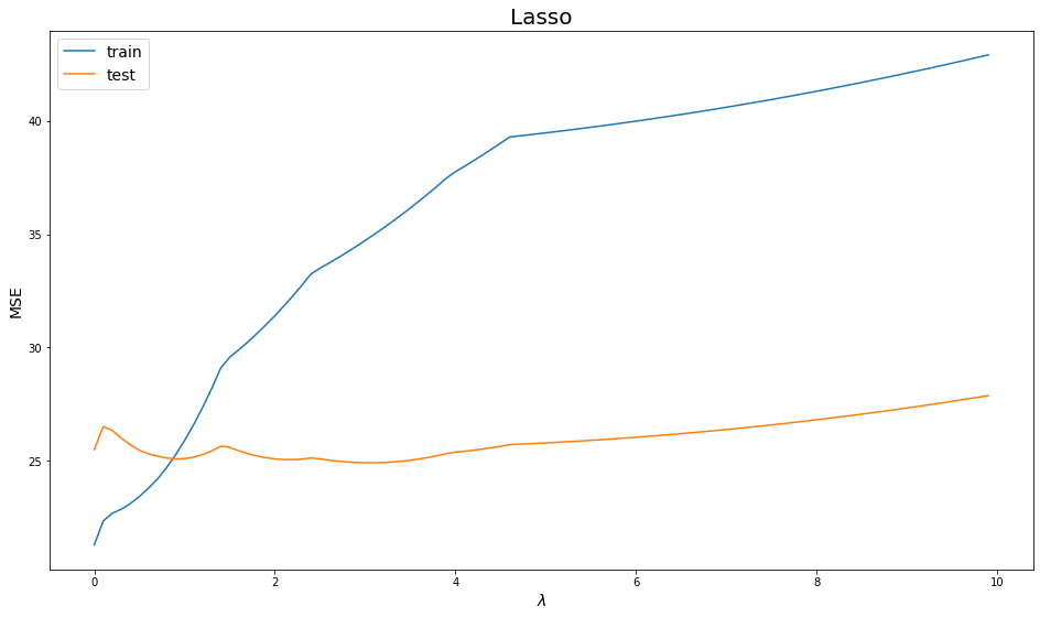
sklearn is already warning us about using 0, the model is to complex it could not even converge to a solution! Just our of curiosty, what about negative $\lambda$? a sort of counter-regularization.

We notice increasing $\lambda$ adds too much regularization that the model starts adding error on both training and testing sets, which means it is underfitting. Using a very low $\lambda$ (e.g. 0.1) seems to gain the least testing error.

lambdas = np.arange(-10, 0.2, step=0.1)

lasso_train, lasso_test = evaluate_model(Lasso, lambdas)
plot_errors(lambdas, lasso_train, lasso_test, "Lasso")

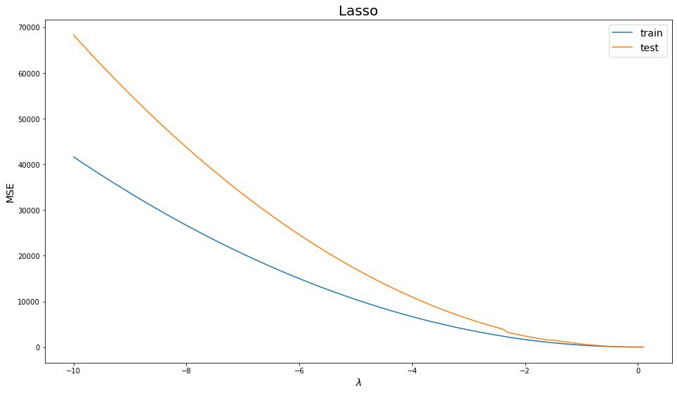
Wow, the error jumped to 4000! Lasso increases the error monotonously with negative $\lambda$ values.

Ridge L2 Regularization

$$\text{Ridge} = RSS + \lambda \sum_{j=1}^k {\beta_j^2}$$

# let's generate different values for lambda from 0 (no-regularization) and (10 too much regularization)
lambdas = np.arange(0, 10, step=0.1)

ridge_train, ridge_test = evaluate_model(Ridge, lambdas)
plot_errors(lambdas, ridge_train, ridge_test, "Ridge")

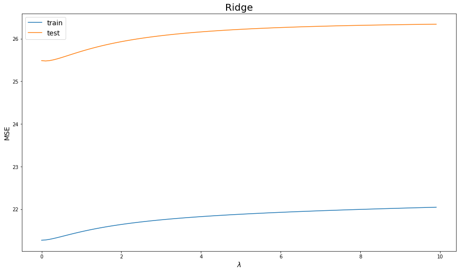
Ridge is noticeably smoother than Lasso, that goes to the fact that the square value introduces a larger error to minimize than just the absolute value, for example ($|-10| = 10$) but ($(-10)^2 = 100$).

lambdas = np.arange(-10, 0.2, step=0.1)

ridge_train, ridge_test = evaluate_model(Ridge, lambdas)
plot_errors(lambdas, ridge_train, ridge_test, "Ridge")

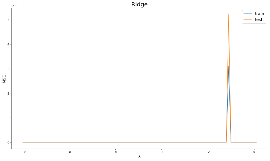
Wow, the error jumped to 1400 then came back to erros similarly small with the positive $\lambda$s.

Elastic Net Regularization

$$\text{ElasticNet} = RSS + \lambda \sum_{j=1}^k {(|\beta_j| + \beta_j^2)}$$

# let's generate different values for lambda from 0 (no-regularization) and (10 too much regularization)
lambdas = np.arange(0, 10, step=0.1)

elastic_train, elastic_test = evaluate_model(ElasticNet, lambdas)
plot_errors(lambdas, elastic_train, elastic_test, "Elastic Net")

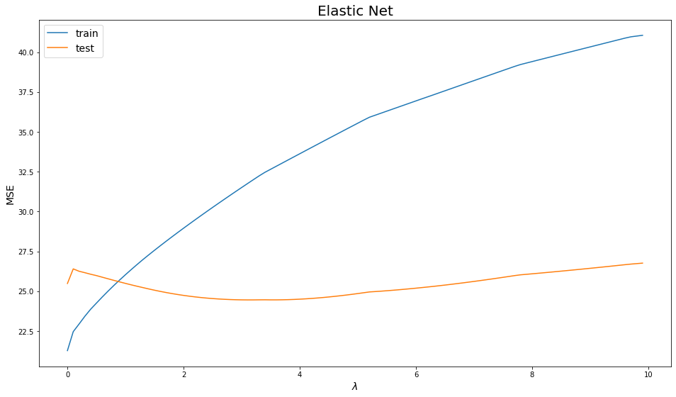
ElasticNet performance if remarkably comparable with Lasso.

lambdas = np.arange(-10, 0.2, step=0.1)

elastic_train, elastic_test = evaluate_model(ElasticNet, lambdas)
plot_errors(lambdas, elastic_train, elastic_test, "Elastic Net")

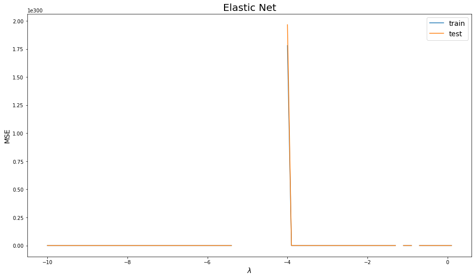
Negative values of $\lambda$ break Elastic Net, so let's not do that.

Regularization Techniques Comparison

Lasso: will eliminate many features, and reduce overfitting in your linear model.
Ridge: will reduce the impact of features that are not important in predicting your y values.
Elastic Net: combines feature elimination from Lasso and feature coefficient reduction from the Ridge model to improve your model’s predictions.