Rectified Linear Unit For Artificial Neural Networks - Part 1 Regression
Introduction
Our brains house a huge network of nearly a 100 billion tiny neural cells (aka neurons) connected by axons.
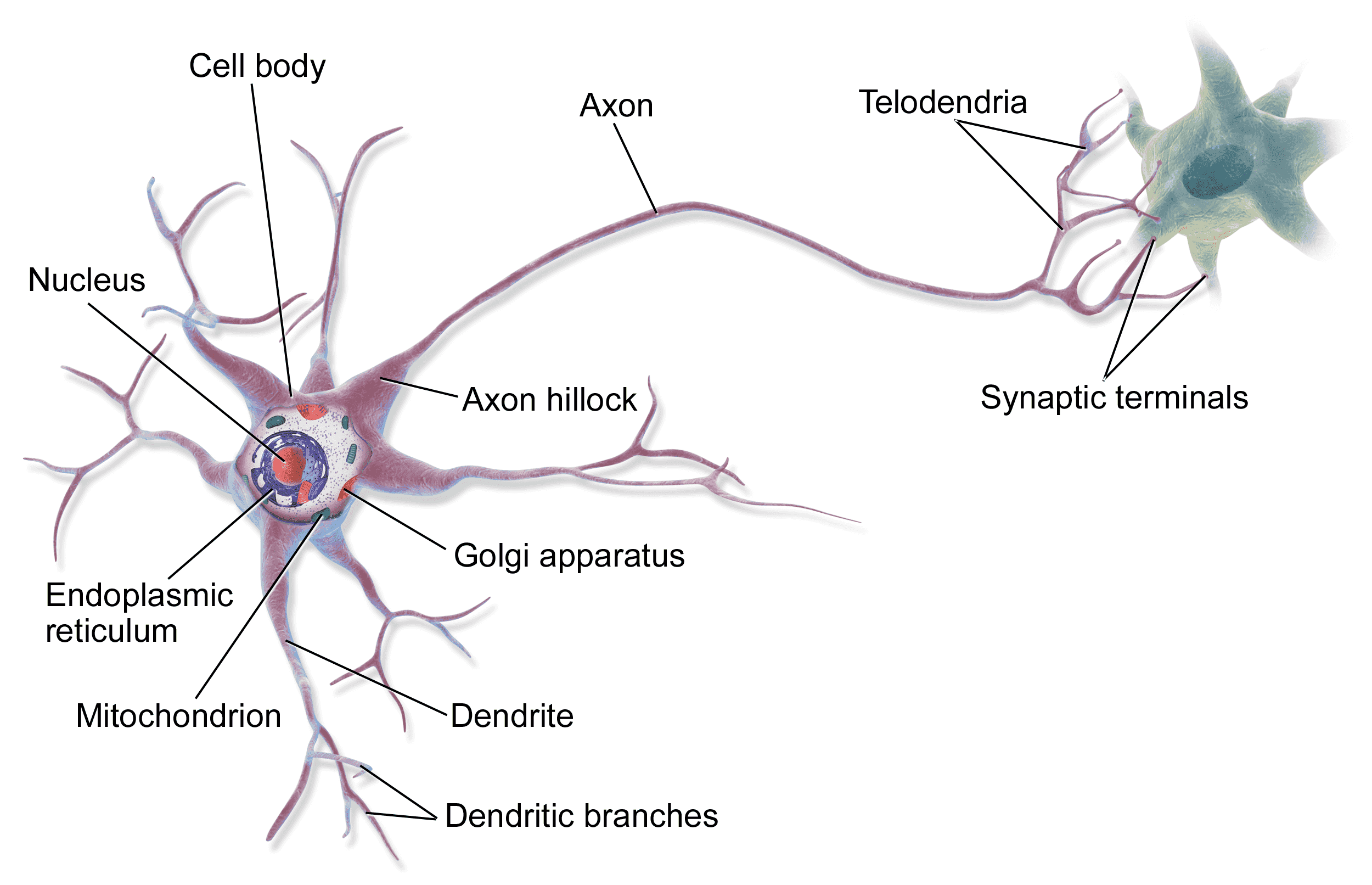
Neural Networks: Neurons communicate by sending electric charges to each other. Neurons only fire an electric charge if they are sufficiently stimulated, in which case the neuron is activated. Through an incredibly intricate scheme of communication, each pattern of electric charges fired throughout the brains are translated into our neural activities, whether it is to taste a burger, tell a joke, or enjoy a scenery.
Learning: To activate a neuron, sufficient electric charge is required to go through the axon of that neuron. Some axons are more conductive of electricity than others. If there is too much conductivity in a brain, the person could have seizure and probably death. However, brains are designed to minimize the enerjy consumption. The learning happens in our brains by making the neurons responsible for a certain act or thought more conductive and more connected. So everytime we play a violin for example, the part of our brain that plays the violin gets more and more connected and conductive. This in turn makes the electric charges in this area travel much faster, which translates into faster responses. In other words, playing violin becomes like a "second hand". As the proverb goes "practice makes perfect".
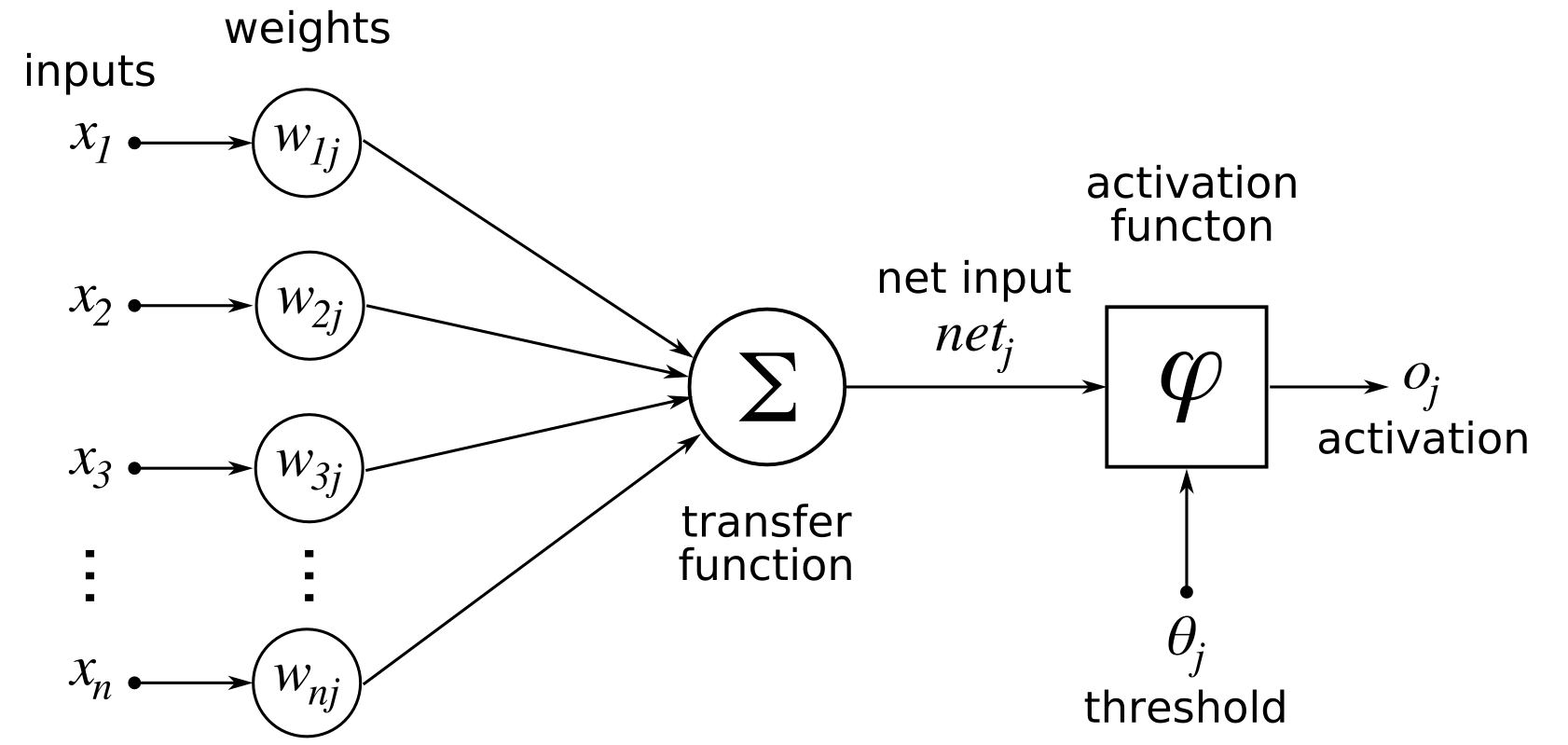
Artificial Neural Networks (ANN): This idea is simulated in artificial neural networks where we represent our model as neurons connected with edges (similar to axons). The value of a neuron is simply the sum of the values of previous neurons connected to it weighted by the weights of their edges. Finally the neuron is passed through a function to decide how much it should be activated, which is called an activation function.
ANN and Linear Algebra: ANNs are just a fancy representation of matrix multiplication. Each layer in an ANN is simply a vector, while the weights connecting layers are matrices. Formally, we refer them as tensors, as they can vary in their dimensionality. For example, consider the following input:
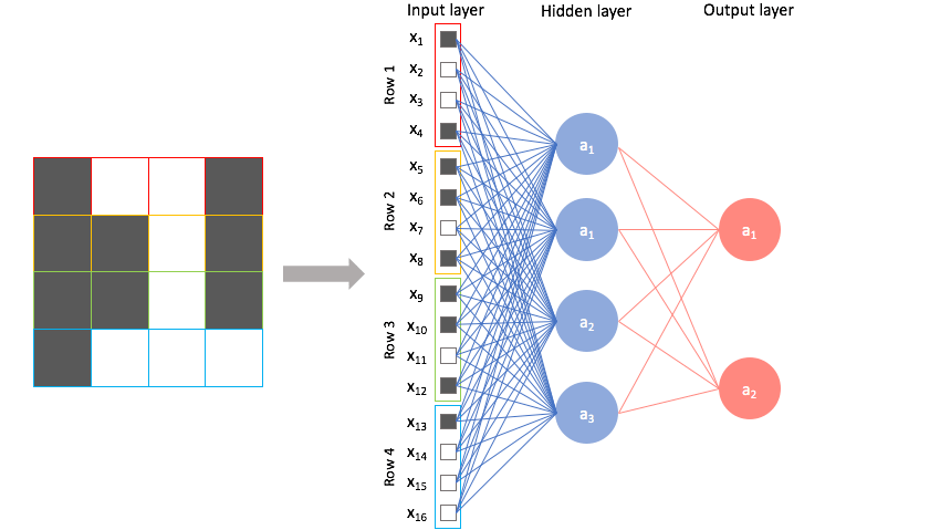
We have 3 layers, input, hidden, and output. The input layer is simply the 16-dimensional feature vector of the input image. The hidden layer is a 4-dimensional vector of neurons that represent a more abstracted version of the raw input features. We obtain this hidden layer by simply multiplying the input vector with the weights matrix $W_1$, which is 16x4. Similarly, the output layer is obtained by multiplying the hidden layer by another weights matrix $W_2$, which is 4x2.
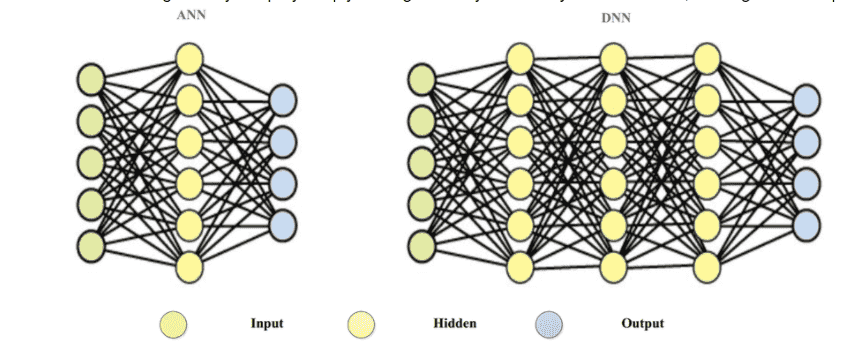
Deep Neural Networks: these ANNs can get really deep by simply adding as many hidden layers as we want, making them Deep Neural Networks (DNN)
Training a neural network: To extremely simply things to an unfair degree, we basically start with random values for weights. We travel through the layers to the output layer, which houses our predictions. We calculate the error of our predictions, and accordingly slightly fix our weight matrices. We repeat until the weights stop changing much. This is not doing justice for the neatness of the gradient descent and back propagation algorithms, but it is enough for using neural networks in applications. Here is a GIF for an error (aka loss) getting smaller and smaller as the weights are modified.
Activation Function (ReLU)
We apply activation functions on hidden and output neurons to prevent the neurons from going too low or too high, which will work against the learning process of the network. Simply, the math works better this way.
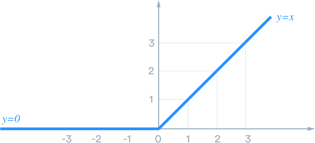
The most important activation function is the one applied to the output layer. If the NN is applied to a regression problem, then the output should be continous. For the sake of demonstration, we are using the Boston house-prices dataset. A house price cannot be negative. We force this rule by using one of the most intuitive and useful activation functions: Rectified Linear Unit. The only thing it does is; if the value is negative, set it to zero. Yub, that's it.
import matplotlib.pyplot as plt
import numpy as np
import pandas as pd
import tensorflow as tf
from sklearn.datasets import load_boston
from sklearn.metrics import mean_absolute_error, mean_squared_error, r2_score
from sklearn.model_selection import train_test_split
from tensorflow.keras.layers import Dense, Dropout, Input
from tensorflow.keras.models import Model

# ensuring that our random generators are fixed so the results remain reproducible
tf.random.set_seed(42)
np.random.seed(42)
data = load_boston()
X = data["data"]
y = data["target"]
df = pd.DataFrame(X, columns=data["feature_names"])
df["PRICE"] = y
df
X_train, X_test, y_train, y_test = train_test_split(X, y, random_state=42)
Relu Activation Function in Python
input_shape = X.shape[1] # number of features, which is 13
# this is regression
# so we only need one neuron to represent the prediction
output_shape = 1
# we set up our input layer
inputs = Input(shape=(input_shape,))
# we add 3 hidden layers with diminishing size. This is a common practice in designing a neural network
# as the features get more and more abstracted, we need less and less neurons.
h = Dense(16, activation="relu")(inputs)
h = Dense(8, activation="relu")(h)
h = Dense(4, activation="relu")(h)
# and finally we use the ReLU activation function on the output layer
out = Dense(output_shape, activation="relu")(h)
model = Model(inputs=inputs, outputs=[out])
model.summary()
We use MSE as the error we are trying to minimize. $$MSE=\frac{1}{n}\sum^n_{i=1}{(y_i-\hat{y_i})^2}$$
Adam is just an advanced version of gradient descent used for optimization. It is relatively faster than other optimizer algorithms. The details are just for another day.
model.compile(optimizer="adam", loss="mean_squared_error")
We fit our model for 4 epochs, where each epoch is a full pass on the entire training data. Epochs are different from learning iterations, as we can do an iteration on batches of the data. However, an epoch passes everytime the model has iterated on all the training data.
H = model.fit(
    x=X_train,
    y=y_train,
    validation_data=(
        X_test, y_test
    ),
    epochs=40,
)
fig = plt.figure(figsize=(16, 9))
plt.plot(H.history["loss"], label="loss")
plt.plot(H.history["val_loss"], label="validation loss")
plt.show()
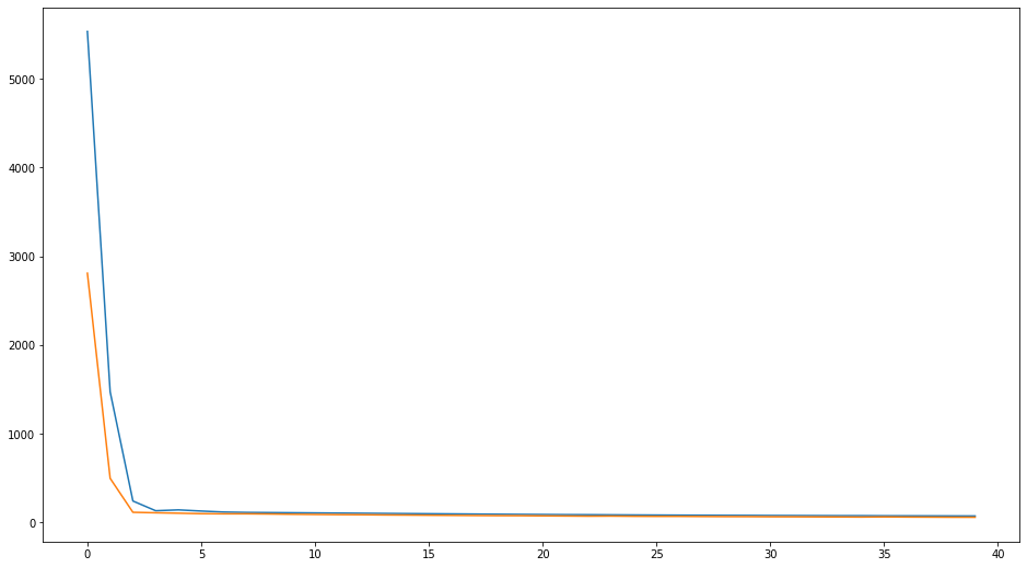
We notice both the training and testing error plumment quickly in the first few epochs, and converge soon after that. Let's explore the data distribution to better understand how well is the performance.
import seaborn as sns
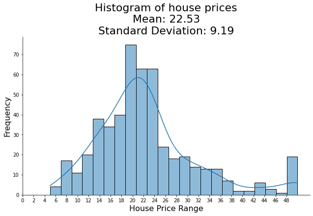
sns.displot(x=y, kde=True, aspect=16/9)
# Add labels
plt.title(f'Histogram of house prices\nMean: {round(np.mean(y), 2)}\nStandard Deviation: {round(np.std(y), 2)}', fontsize=22)
plt.xlabel('House Price Range', fontsize=16)
plt.ylabel('Frequency', fontsize=16)
plt.xticks(np.arange(0, 50, 2))
plt.show()
y_pred = model.predict(X_test)
print(f"RMSE: {np.sqrt(mean_squared_error(y_test, y_pred))}")
print(f"MAE: {mean_absolute_error(y_test, y_pred)}")
print(f"R2: {r2_score(y_test, y_pred)}")
While the data seem to be normally distributed, RMSE is less than one standard deviation. This indicates a good performance of the model!
Related Notebooks
- Activation Functions In Artificial Neural Networks Part 2 Binary Classification
- How To Code RNN and LSTM Neural Networks in Python
- For Loop In R
- Generative Adversarial Networks
- Machine Learning Linear Regression And Regularization
- Lasso and Ridge Linear Regression Regularization
- Regularization Techniques in Linear Regression With Python
- How To Solve Linear Equations Using Sympy In Python
- ERROR Could not find a version that satisfies the requirement numpy==1 22 3