How To Use R Dplyr Package

Contents

1. Introduction
2. Installation
3. Loading the dplyr package with library()
4. Pipes in dplyr
5. The five core verbs of dplyr
   1. filter()
   2. select()
      • select() - dropping one column
      • select() - dropping two or more columns
   3. mutate()
      • mutate_if()
      • mutate_at()
   4. summarise()
   5. arrange()
6. Other useful functions in the dplyr package
   1. group_by()
   2. left_join()
   3. right_join()
   4. full_join()
   5. inner_join()
7. An exercise in data wrangling - how to make a grouped boxplot
   1. melt()
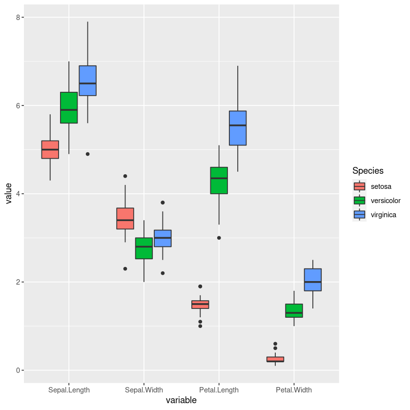
   2. Generating the grouped boxplot with ggplot2

Introduction

The dplyr package is the fundamental package of the wider tidyverse in R. Functions of the dplyr package, in this particular package known as "verbs", are used to manipulate data into a suitable format for subsequent data analysis.

Installation

Before using dplyr it is necessary to install it, since it is not a part of base R. The dplyr package is hosted in the CRAN repository. Any package from the CRAN repository can be installed using the function install.packages().

In the case of dplyr, we will pass it as an argument for install.packages() and run it. {r, eval=FALSE} install.packages("dplyr") Alternatively, we can install the tidyverse collection of packages, which will also include dplyr.

install.packages("tidyverse")

Tip:

This is a useful chunk of code to make sure all the packages you want to use are installed if they are not already installed.

Loading the dplyr package with library()

Now that we have the dplyr package installed we need to load it to our R workspace. For this purpose we can use the library() function. If installed correctly, the message "Attaching package: ‘dplyr’" will appear.

Pipes in dplyr

When reading R code that uses functions from dplyr, you will almost certainly encounter this string of symbols: %>% This is an operator used to pipe the output from one function to the input of another function. For example:

Here we have used the %>% operator to pipe the Sepal.Length column into the function mean(). Writing code in this way provides for a natural and logical flow of operations.

Tip: In order to instantly type the %>% operator, press down Ctrl + Shift + M keys simultaneously.

The five core verbs of dplyr

filter()

The filter() function of dplyr is used to extract rows, based on a specified condition. For example, in the iris dataset, we want to extract only the rows belonging to the "setosa" species.

The result is a dataframe with rows belonging only to the "setosa" species.

select()

Just as the filter() function extracts rows, the select() function extracts columns from a dataframe based on specified condition. Here we can extract columns based on name, the Sepal.Length and Petal.Length columns.

select() - dropping one column

The select() function can also be used to drop columns from a dataframe. Maybe we would like to have a dataframe with only numerical values. In the case of the iris dataset, the solution would be to drop the species column. We can use the logical NOT operator in R, the ! symbol. The following code can be read as follows: "From the iris dataset, select all columns that are not the species column".

Note that the above result can be achieved like this as well, but it is not as elegant.

select() - dropping two or more columns

Here we use the same logic as with dropping one column, expect we will apply the ! operator to a vector of columns we want dropped. As a reminder, the c() is a function that returns a vector. In this example we want to drop the sepal lengths and widths columns.

mutate()

The mutate() function is useful for adding new columns to a dataframe, which will have the results of operations on already existing columns. For example, in the iris_sepal_petal_length dataframe we have created in the previous example, the lengths are given in centimeters and now we would like to add columns with lengths given in inches.

mutate_if()

The mutate_if() function checks if a certain condition is met before applying the transforming operation on the column. In the iris dataset numerical values are given as doubles (number with a decimal). Now imagine if we want to convert the iris dataset to integers, lets try to use mutate() first.

Error in Math.data.frame(structure(list(Sepal.Length = c(5.1, 4.9, 4.7, : non-numeric variable(s) in data frame: Species Traceback:

1. Math.data.frame(structure(list(Sepal.Length = c(5.1, 4.9, 4.7, . 4.6, 5, 5.4, 4.6, 5, 4.4, 4.9, 5.4, 4.8, 4.8, 4.3, 5.8, 5.7,

Oh no, we have an error. The round() function seemed to work fine until it encountered the non-numeric species column. We could drop this column as we showed with select(), but instead we can use mutate_if() to check if a column is numeric before trying to change it.

mutate_at()

We see in the previous example that the petal width column rounds down to zero, lets round all other numerical columns, but keep the petal width column as a double. The mutate_at() function allows us to specify on exactly which colums we want to perform some operation.

summarise()

The summarise() function is used to provide different summary statistics from a dataframe. For example, we want to summarise the means of the petal and sepal lenghts from our iris_sepal_petal_length dataframe.

arrange()

The arrange() function sorts rows of dataframe based on the values in one (or more) of its columns. By default it sorts from lowest to highest value.

We could also arrange rows based on values in two or more columns.

To arrange rows in a descending order we can use the desc() function from dplyr package.

Other useful functions in the dplyr package

group_by()

Sometimes you want certain operations performed on groups in your dataset. Previously we used the summarise() to get column means of all our iris data. Now we would like to get the species means. Logically we can first group our data by the species column.

Compare this result with the result of the summarise() function in chapter 4.4 summarise(). Note that grouping data does not change how your data looks, only how it is interpreted by other functions.

left_join()

The left_join() function is used to join two dataframes based on matches in a common column between them. The function returns all rows from the left dataframe, and all columns from both dataframes. Rows in the left with no match in right will have NA (missing) values in the new columns. We can look at two dataframes, band_members and band_instruments.

We see that both dataframes have the name column in common, and it is by this column that we will join them.

Notice that Mick has NA in the instruments column, because he does not have a match in the right dataframe.

right_join()

The right_join() works simmilarly as 5.2 left_join() only the right dataframe is given priority, meaning if the rows in the left dataframe do not have a match in right they will have NA values in the new columns.

full_join()

The full_join() function returns all rows and columns from both dataframes. If no matching values are found NAs are placed.

{r}
band_members %>% full_join(band_instruments)

inner_join()

The inner_join() function return all rows and columns from both dataframes that have a match, dropping all rows that have a mishmatch.

An exercise in data wrangling - how to make a grouped boxplot

We will use the iris dataset for this example.

Here we see a dataframe in what is called a wide format, meaning every observation, in this case a individual iris plant has its measurements in its own row, and every variable has its own column. In order to make a grouped boxplot we need to change this dataframe into a long format.

melt()

We can use the melt() function to convert the iris dataframe into a long format. The long format has for each data point as many rows as the number of variables and each row contains the value of a particular variable for a given data point. The melt() function is part of the reshape2 package so we will first load it.

Generating the grouped boxplot with ggplot2

The package ggplot2 contains powerful tools for visualizing data in R, and will be covered in depth in a subsequent guide. For now we will just showcase its capabillites.