How to Visualize Data Using Python - Matplotlib

Introduction to Visualization

Data Science is one of the trending topics in this current generation. Big Data is a subset of Data Science where petabytes of huge data are handled every second – like Facebook & Twitter. When it comes to a huge number of data to handle human brain struggles.

One way how human handles this situation is through simplifying huge data in a form that he can understand – Charts & Graphs. This is the situation where Data Visualization comes into play.

Python is a human-friendly programming language for data visualization. Different frameworks/libraries can be used with Python for visualization purposes such as Matplotlib, Seaborn, GGPlot and so on. However, in this article, we focus on how to use Matplotlib library for data visualization.

Scope of the Article

This article will initially explain an overview of a “figure” generated by Matplotlib and extend towards the use of its subclasses – pyplot & pylab. Eventually, we will instruct how to plot and play around with the graph using Python – Matplotlib, with basic functions, give you a kick-start.

Prerequisites – Python Version 3.6 or above & Python IDE.

Parts of Figure

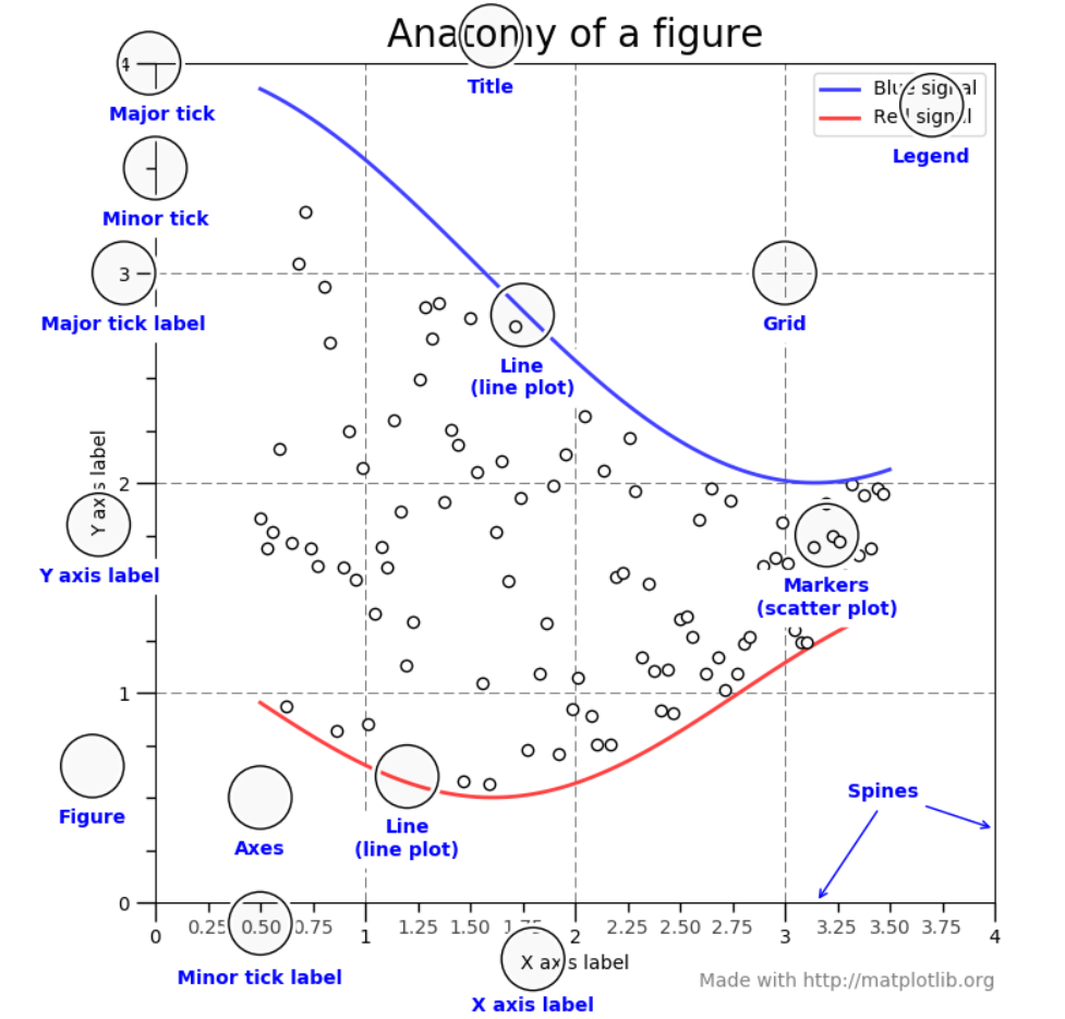
A figure keeps track of Axes, Artists & the Canvas. A figure can have any number of axes; at least one.

Axes is the region of the image displayed along with the data space. A figure can have multiple axes, but an axes object can only be in one figure. There are two axis objects that are responsible for data limits in an axes object.

Axis is the number line of the figure that sets the graph limit as well as generate the ticks & tick-labels.

Artist is everything you can see on the figure – the combination of figure, axes & axis objects.  

What is the Relationship between Matplotlib, Pyplot & Pylab

Consider Matplotlib as a whole package, then pyplot is a module of that package. Another module for importing both pyplot & numpy in a single namespace together is known as pylab. Due to namespace pollution, pylab is not encouraged to use; instead, go with pyplot.

How to Plot with Python - Matplotlib

It doesn’t matter what graph or chart you create with Matplotlib. The bottom line of any visualization is, it will inherit from the concept of figure, axes, axis & artist. From this time forth, we will discuss how to plot a graph with Python.

For demonstration purposes, I’ll be using a dummy dataset downloaded from GitHub (You may replace the data with your own). This dataset refers to the prices of gas from 1990 to 2007 in 8 different countries. Also, we will be using numpy & panda libraries to assist with the analysis.

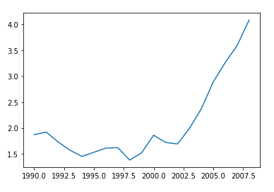
How to Plot a Graph?

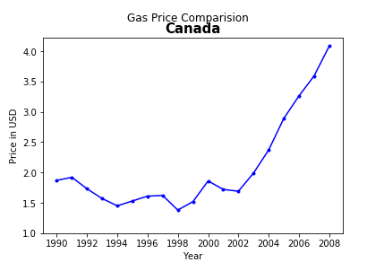
First, we will create a line plot to visualize the gas price in Canada. You can use the matplotlib.pyplot.plot() function to plot a line chart. According to the visual outcome in the below figure, it can be clearly seen that after the year 2002 the price has a gradual increment.

import matplotlib.pyplot as plt
import numpy as np
import pandas as pd

gasPrice = pd.read_csv('gas_prices.csv')
plt.plot(gasPrice.Year, gasPrice.Canada)

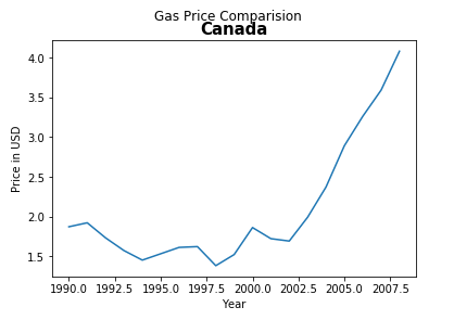
How to add a Title to the graph?

You can add two types of titles to the graphs. One, a title to the figure which is centered – matplotlib.pyplot.suptitle(). Two, a title for the axes - matplotlib.pyplot.title(). Make sure you use relevant naming titles as it will be important to the user to understand the graph.

The difference between suptitle() & title() is the position they stick. The title() somewhat sticks close with axes slightly below the suptitle(). Besides, using title() function you have the option to align, change the font style, color, size and so on.

Moreover, you can set the title to x-axis & y-axis using the  matplotlib.pyplot.xlabel() and matplotlib.pyplot.ylable() functions respectively.

import matplotlib.pyplot as plt
import numpy as np
import pandas as pd

gasPrice = pd.read_csv('gas_prices.csv')
plt.plot(gasPrice.Year, gasPrice.Canada)
plt.suptitle('Gas Price Comparison')
plt.title('Canada', fontdict={'fontsize':15,'fontweight':'bold'})
plt.xlabel('Year')
plt.ylabel('Price in USD')

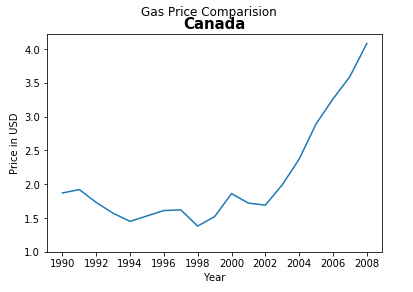
How to set Tick to the graph?

Displaying ticks are important as the values displayed adds more meaning to the visual. Matplotlib automatically selects the ticks if we haven’t instructed it. In our case, the year is displayed in decimal which is not the right way. So, you can use the matplotlib.pyplot.xticks() & matplotlib.pyplot.yticks() functions to set them meaningfully.

import matplotlib.pyplot as plt
import numpy as np
import pandas as pd

gasPrice = pd.read_csv('gas_prices.csv')
plt.plot(gasPrice.Year, gasPrice.Canada)
plt.suptitle('Gas Price Comparison')
plt.title('Canada', fontdict={'fontsize':15,'fontweight':'bold'})
plt.xlabel('Year')
plt.ylabel('Price in USD')
plt.xticks([1990,1992,1994,1996,1998,2000,2002,2004,2006,2008])
plt.yticks([1,1.5,2,2.5,3,3.5,4])

How to set Dot-Marker?

The current blue line is the default line which could be added more meaning by dot-marker. Giving a dot-marker to the line will make the graph visually more attractive. Simply, you can add an attribute (‘b.-’) to matplotlib.pyplot.plot() function. There are plenty of other markers such as point-marker, pixel-marker, circle-marker and so on are available in the official site. You can select any meaningful marker you prefer.

import matplotlib.pyplot as plt
import numpy as np
import pandas as pd

gasPrice = pd.read_csv('gas_prices.csv')
plt.plot(gasPrice.Year, gasPrice.Canada,'b.-')
plt.suptitle('Gas Price Comparison')
plt.title('Canada', fontdict={'fontsize':15,'fontweight':'bold'})
plt.xlabel('Year')
plt.ylabel('Price in USD')
plt.xticks([1990,1992,1994,1996,1998,2000,2002,2004,2006,2008])
plt.yticks([1,1.5,2,2.5,3,3.5,4])

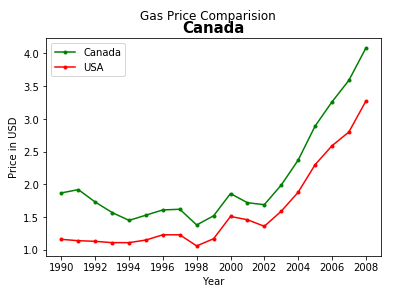
How to display Legend?

In order to display the legend, there should be a label attribute within matplotlib.pyplot.plot() function. Then, you can use matplotlib.pyplot.legend() function to display the label. Legends work in handy when you want to compare 2 or more different lines. In this example, I will add another country to display the legend. Also, it is recommended to change the color of the lines as well.

import matplotlib.pyplot as plt
import numpy as np
import pandas as pd

gasPrice = pd.read_csv('gas_prices.csv')
plt.plot(gasPrice.Year, gasPrice.Canada,'b.-',label = 'Canada',color='green')
plt.plot(gasPrice.Year, gasPrice.USA,'b.-',label = 'USA',color='red')
plt.suptitle('Gas Price Comparison')
plt.title('Canada', fontdict={'fontsize':15,'fontweight':'bold'})
plt.xlabel('Year')
plt.ylabel('Price in USD')
plt.xticks([1990,1992,1994,1996,1998,2000,2002,2004,2006,2008])
plt.yticks([1,1.5,2,2.5,3,3.5,4])
plt.legend()

How to Change Figure Size?

You can change the size of the figure in Inches using matplotlib.pyplot.figure() function. You can set the size using a figsize attribute, as well as you can additionally set the dpi of the image. The output will be the figure displayed according to the size set in the function.

import matplotlib.pyplot as plt
import numpy as np
import pandas as pd

gasPrice = pd.read_csv('gas_prices.csv')
plt.plot(gasPrice.Year, gasPrice.Canada,'b.-',label = 'Canada',color='green')
plt.plot(gasPrice.Year, gasPrice.USA,'b.-',label = 'USA',color='red')
plt.suptitle('Gas Price Comparison')
plt.title('Canada', fontdict={'fontsize':15,'fontweight':'bold'})
plt.xlabel('Year')
plt.ylabel('Price in USD')
plt.xticks([1990,1992,1994,1996,1998,2000,2002,2004,2006,2008])
plt.yticks([1,1.5,2,2.5,3,3.5,4])
plt.legend()
plt.figure(figsize=(10,12), dpi=100)

How to Save the Plot?

Matplotlib also provides the convenience to save the plots on your computer. You can use matplotlib.pyplot.savefig() function to achieve this task. Make sure to name your image and instead of the name you can give the location to save as well.

import matplotlib.pyplot as plt
import numpy as np
import pandas as pd

gasPrice = pd.read_csv('gas_prices.csv')
plt.plot(gasPrice.Year, gasPrice.Canada,'b.-',label = 'Canada',color='green')
plt.plot(gasPrice.Year, gasPrice.USA,'b.-',label = 'USA',color='red')
plt.suptitle('Gas Price Comparison')
plt.title('Canada', fontdict={'fontsize':15,'fontweight':'bold'})
plt.xlabel('Year')
plt.ylabel('Price in USD')
plt.xticks([1990,1992,1994,1996,1998,2000,2002,2004,2006,2008])
plt.yticks([1,1.5,2,2.5,3,3.5,4])
plt.legend()
plt.figure(figsize=(10,12), dpi=100)
plt.savefig('Gas Price Comparision (Canada & USA).png', dpi=300)

What else can you do with Matplotlib?

In addition, you can plot other types of graphs such as a bar chart, pie chart, histogram, box-plots and so on. Functions you use, have plenty of other attributes you can insert into. You can explore them from the official Matplotlib website. Try to play around with all the available options to practice well if you want to become a professional data analyst.

Conclusion

All the above-mentioned guidelines are just basic for you to get-start with plotting graphs using Python. In the real world, the data set used are very large compared to the example. Knowledge of statistics is very important for data visualization with Python. Once you know the basics, yes you can move towards advanced visualization techniques.