How To Run Logistic Regression In R

For this post I will use Weely stock market S&P data between year 1990 and 2010. I downloaded the data from following link...

app.quadstat.net/dataset/r-dataset-package-islr-weekly

How to read csv data in R

In [1]:
df = read.csv('data/dataset-95529.csv',header = TRUE)

Let us check the number of rows in our R dataframe using nrow.

In [2]:
nrow(df)
1089

For columns, we can use ncol(dataframe)

In [3]:
ncol(df)
9

Data has 9 columns. All the columns are self explanatory except lag1,lag2,lag3,lag4,lag5 which are percentage returns for previous weeks.

Let us look at the summary of our data. We can use summary function in R which takes the dataframe and prints valuable summary.

In [4]:
summary(df)
      Year           Lag1               Lag2               Lag3         
 Min.   :1990   Min.   :-18.1950   Min.   :-18.1950   Min.   :-18.1950  
 1st Qu.:1995   1st Qu.: -1.1540   1st Qu.: -1.1540   1st Qu.: -1.1580  
 Median :2000   Median :  0.2410   Median :  0.2410   Median :  0.2410  
 Mean   :2000   Mean   :  0.1506   Mean   :  0.1511   Mean   :  0.1472  
 3rd Qu.:2005   3rd Qu.:  1.4050   3rd Qu.:  1.4090   3rd Qu.:  1.4090  
 Max.   :2010   Max.   : 12.0260   Max.   : 12.0260   Max.   : 12.0260  
      Lag4               Lag5              Volume            Today         
 Min.   :-18.1950   Min.   :-18.1950   Min.   :0.08747   Min.   :-18.1950  
 1st Qu.: -1.1580   1st Qu.: -1.1660   1st Qu.:0.33202   1st Qu.: -1.1540  
 Median :  0.2380   Median :  0.2340   Median :1.00268   Median :  0.2410  
 Mean   :  0.1458   Mean   :  0.1399   Mean   :1.57462   Mean   :  0.1499  
 3rd Qu.:  1.4090   3rd Qu.:  1.4050   3rd Qu.:2.05373   3rd Qu.:  1.4050  
 Max.   : 12.0260   Max.   : 12.0260   Max.   :9.32821   Max.   : 12.0260  
 Direction 
 Down:484  
 Up  :605  


In our summary above, we can see that last column is "Direction". Out of 1089 entries, 484 times it tells us that market had negative return and 605 times positive return.

We can use this data to train our model to predict if the weekly return would be positive or negative.

How to run Logistic Regression in R

Since the variable "Direction" is categorical. We can try using Logistic Regression. Logistic regression is similar in nature to linear regression. In R it is very easy to run Logistic Regression using glm package. glm stands for generalized linear models. In R glm, there are different types of regression available. For logistic regression, we would chose family=binomial as shown below.

In [5]:
glm.fit <- glm(Direction ~ Lag1 + Lag2 + Lag3 + Lag4 + Lag5 + Volume, family = binomial, data = df)

glm.fit is our model. glm is the package name. Direction is the output variable. To right of symbol ~ everything else is independent variables.

We can look at the summary of our logistic model using function summary.

In [6]:
summary(glm.fit)
Call:
glm(formula = Direction ~ Lag1 + Lag2 + Lag3 + Lag4 + Lag5 + 
    Volume, family = binomial, data = df)

Deviance Residuals: 
    Min       1Q   Median       3Q      Max  
-1.6949  -1.2565   0.9913   1.0849   1.4579  

Coefficients:
            Estimate Std. Error z value Pr(>|z|)   
(Intercept)  0.26686    0.08593   3.106   0.0019 **
Lag1        -0.04127    0.02641  -1.563   0.1181   
Lag2         0.05844    0.02686   2.175   0.0296 * 
Lag3        -0.01606    0.02666  -0.602   0.5469   
Lag4        -0.02779    0.02646  -1.050   0.2937   
Lag5        -0.01447    0.02638  -0.549   0.5833   
Volume      -0.02274    0.03690  -0.616   0.5377   
---
Signif. codes:  0 ‘***’ 0.001 ‘**’ 0.01 ‘*’ 0.05 ‘.’ 0.1 ‘ ’ 1

(Dispersion parameter for binomial family taken to be 1)

    Null deviance: 1496.2  on 1088  degrees of freedom
Residual deviance: 1486.4  on 1082  degrees of freedom
AIC: 1500.4

Number of Fisher Scoring iterations: 4

summary has lot of information. We can selectively look at the information too. To check what are the available fields to query in the summary, do names(summary(model)).

In [7]:
names(summary(glm.fit))
  1. 'call'
  2. 'terms'
  3. 'family'
  4. 'deviance'
  5. 'aic'
  6. 'contrasts'
  7. 'df.residual'
  8. 'null.deviance'
  9. 'df.null'
  10. 'iter'
  11. 'deviance.resid'
  12. 'coefficients'
  13. 'aliased'
  14. 'dispersion'
  15. 'df'
  16. 'cov.unscaled'
  17. 'cov.scaled'

Let us save the summary in to new variable and then query some of the above fields.

In [8]:
glm.sum <- summary(glm.fit)

Let us query coeffients of our logistic regression model.

In [9]:
glm.sum$coefficients
A matrix: 7 × 4 of type dbl
EstimateStd. Errorz valuePr(>|z|)
(Intercept) 0.266864140.08592961 3.10561340.001898848
Lag1-0.041268940.02641026-1.56260990.118144368
Lag2 0.058441680.02686499 2.17538390.029601361
Lag3-0.016061140.02666299-0.60237600.546923890
Lag4-0.027790210.02646332-1.05014090.293653342
Lag5-0.014472060.02638478-0.54850060.583348244
Volume-0.022741530.03689812-0.61633300.537674762

Above matrix is very important. The last column Pr(>|z|) is a p-value. If Pr(>|z|) is less than 0.05, it means parameter is significant and tells us that co-efficient estimate is significantly different from zero. All the parameters which have Pr(>|z|) less than 0.05 are significant. In the above table, we can see that intercept, Lag2 have p-value less than 0.05, there are significant parameters.

Let us use our model now to predict. In practice we should train our model on training data, then test it on unseen data. For now we are skipping that part. We would take our previous model which has already seen our test data.

In [10]:
glm.probs = predict(glm.fit,type="response")

Ok, our predict model is ready. Remember this is logistic regression, so our model would generate probabilities. We would mark our return as Up if probability is greater than 0.5 otherwise down.

In [11]:
glm.pred = rep("Down",length(glm.probs)) 
glm.pred[glm.probs > 0.5] = "Up"

Let us now look at the output in the form of confusion matrix.

In [12]:
table(glm.pred, df$Direction)
        
glm.pred Down  Up
    Down   54  48
    Up    430 557

the above confusion matrix: Error rate (Down) = 430/(430+54) = 88.8% that means 88.8% of predictions about the down days are wrong , for all these days the model has predicted that market will go up. Error rate (Up) = 48/(48+557) = 7.9%, whereas while predicting Up days, the model has done very good job of being wrong only 7.9%

How to run Logistic Regression in R using Deep Learning library H2o

We can improve on our previous Logistic Regression results using deep learning package from H2o library.

Make sure you have h2o installed. If not Check out following tutorial to install h2o.

Once you have h2o installed. Let us import h2o and initialize it.

In [28]:
library(h2o)
h2o.init()

Let us first import our data using h2o.importFile function.

In [15]:
df.h2o <- h2o.importFile('data/dataset-95529.csv')
  |======================================================================| 100%

Let us define a variable to store all the x variables. We would use -match function in R to do that.

In [20]:
xall <- names(df.h2o)[-match(c("Direction"),names(df.h2o))]
In [16]:
head(df.h2o,1)
A data.frame: 1 × 9
YearLag1Lag2Lag3Lag4Lag5VolumeTodayDirection
<dbl><dbl><dbl><dbl><dbl><dbl><dbl><dbl><fct>
119900.8161.572-3.936-0.229-3.4840.154976-0.27Down
In [17]:
head(df[xall],1)
A data.frame: 1 × 8
YearLag1Lag2Lag3Lag4Lag5VolumeToday
<int><dbl><dbl><dbl><dbl><dbl><dbl><dbl>
119900.8161.572-3.936-0.229-3.4840.154976-0.27

This time around, we would test our model against unseen data. Let us split the data in to train, valid and test data using h2o.splitFrame function in R as shown below.

In [18]:
parts <- h2o.splitFrame(df.h2o,c(0.8,0.1),seed=70)
In [19]:
train <- parts[[1]]
valid <- parts[[2]]
test <- parts[[3]]
In [21]:
xall
  1. 'Year'
  2. 'Lag1'
  3. 'Lag2'
  4. 'Lag3'
  5. 'Lag4'
  6. 'Lag5'
  7. 'Volume'
  8. 'Today'

Let us now build our h2o deeplearning model. We would wrap it around with system.time to see the time taken to build the model.

In [22]:
y <- 'Direction'
system.time(m <- h2o.deeplearning(xall,y,train,validation_frame = valid))
  |======================================================================| 100%
   user  system elapsed 
  0.389   0.017   2.534 

Ok, model building was pretty quick. Let us look at the perfomance on validation set.

In [23]:
h2o.performance(m,valid = TRUE)
H2OBinomialMetrics: deeplearning
** Reported on validation data. **
** Metrics reported on full validation frame **

MSE:  0.01028619
RMSE:  0.1014209
LogLoss:  0.03346112
Mean Per-Class Error:  0
AUC:  1
AUCPR:  0.5416667
Gini:  1

Confusion Matrix (vertical: actual; across: predicted) for F1-optimal threshold:
       Down Up    Error    Rate
Down     53  0 0.000000   =0/53
Up        0 72 0.000000   =0/72
Totals   53 72 0.000000  =0/125

Maximum Metrics: Maximum metrics at their respective thresholds
                        metric threshold     value idx
1                       max f1  0.133946  1.000000  39
2                       max f2  0.133946  1.000000  39
3                 max f0point5  0.133946  1.000000  39
4                 max accuracy  0.133946  1.000000  39
5                max precision  1.000000  1.000000   0
6                   max recall  0.133946  1.000000  39
7              max specificity  1.000000  1.000000   0
8             max absolute_mcc  0.133946  1.000000  39
9   max min_per_class_accuracy  0.133946  1.000000  39
10 max mean_per_class_accuracy  0.133946  1.000000  39
11                     max tns  1.000000 53.000000   0
12                     max fns  1.000000 39.000000   0
13                     max fps  0.000000 53.000000  92
14                     max tps  0.133946 72.000000  39
15                     max tnr  1.000000  1.000000   0
16                     max fnr  1.000000  0.541667   0
17                     max fpr  0.000000  1.000000  92
18                     max tpr  0.133946  1.000000  39

Gains/Lift Table: Extract with `h2o.gainsLift(<model>, <data>)` or `h2o.gainsLift(<model>, valid=<T/F>, xval=<T/F>)`

Fron the confustion matrix, we can see model is spot on. Model has been able to predict everything right.

To see the importance of each variable in our model. We can use h2o.varimp_plot() function.

In [24]:
h2o.varimp_plot(m)

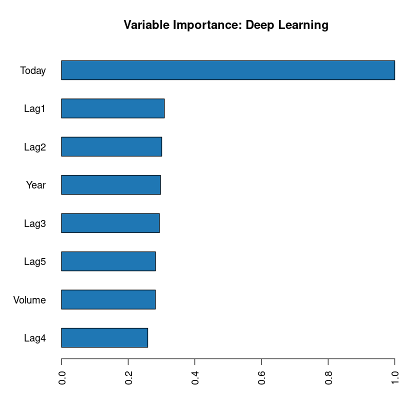
As see see above, variable "Today" (price) is the most important one, followed by Lag1 and so on and soforth.

Let us see now how our model performs work the unseen data. We would feed in test data which is not seen by our model so far yet.

In [25]:
h2o.performance(m,test)
H2OBinomialMetrics: deeplearning

MSE:  0.01311956
RMSE:  0.1145406
LogLoss:  0.05700227
Mean Per-Class Error:  0
AUC:  1
AUCPR:  0.5238095
Gini:  1

Confusion Matrix (vertical: actual; across: predicted) for F1-optimal threshold:
       Down Up    Error    Rate
Down     39  0 0.000000   =0/39
Up        0 63 0.000000   =0/63
Totals   39 63 0.000000  =0/102

Maximum Metrics: Maximum metrics at their respective thresholds
                        metric threshold     value idx
1                       max f1  0.008208  1.000000  32
2                       max f2  0.008208  1.000000  32
3                 max f0point5  0.008208  1.000000  32
4                 max accuracy  0.008208  1.000000  32
5                max precision  1.000000  1.000000   0
6                   max recall  0.008208  1.000000  32
7              max specificity  1.000000  1.000000   0
8             max absolute_mcc  0.008208  1.000000  32
9   max min_per_class_accuracy  0.008208  1.000000  32
10 max mean_per_class_accuracy  0.008208  1.000000  32
11                     max tns  1.000000 39.000000   0
12                     max fns  1.000000 33.000000   0
13                     max fps  0.000000 39.000000  71
14                     max tps  0.008208 63.000000  32
15                     max tnr  1.000000  1.000000   0
16                     max fnr  1.000000  0.523810   0
17                     max fpr  0.000000  1.000000  71
18                     max tpr  0.008208  1.000000  32

Gains/Lift Table: Extract with `h2o.gainsLift(<model>, <data>)` or `h2o.gainsLift(<model>, valid=<T/F>, xval=<T/F>)`

Ok, our model has done pretty well. Predicting everything correct. We can also look at our confusion matrix using h2o.confusionMatrix as shown below.

In [26]:
h2o.confusionMatrix(m,test)
A H2OTable: 3 × 4
DownUpErrorRate
<dbl><dbl><dbl><fct>
Down39 00 =0/39
Up 0630 =0/63
Totals39630 =0/102

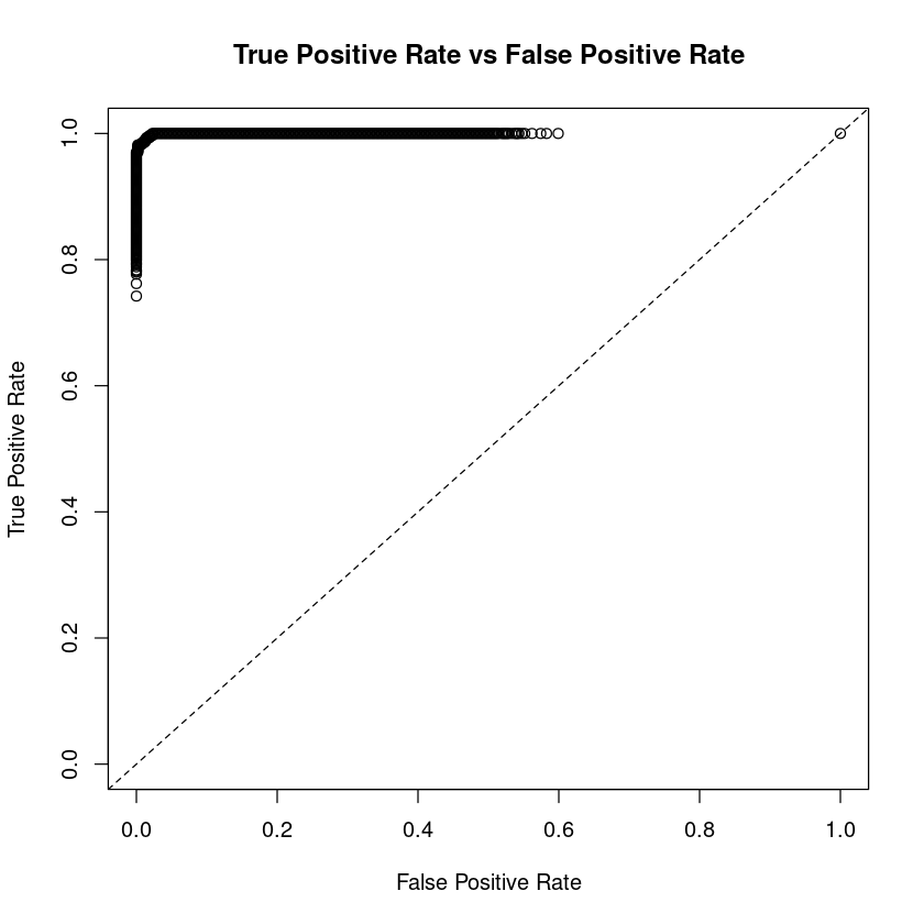
Let us end this post by plotting ROC curves. ROC curves plot "True Positive Rate" vs "Fals Positive Rate".

  1. True Positive Rate (Sensitivity) - The probability of target = Y when its true value is Y
  2. False Positive Rate (Specificity) - The probability of Target = Y when its true value is not Y

Ideally the ratio between ROC curve and diagonal line should be as big as possible which is what we got in our model. The plot is shown below.

In [27]:
perf <- h2o.performance(m, df.h2o)
plot(perf, type="roc")

Wrap Up!

In this post, I have demonstrated how to run logistic regression with R. Also exposed you to machine learning library H2o and its usage for running deep learning models.