How To Use VLOOKUP Function In Excel
Let’s say you are assigned to find the customer details of a specific customer ID or number from a customer data sheet that you have. How will you retrieve the data easily?
You can try to “find” or “search” it using Find and Replace feature (Ctrl+F). You can copy the customer ID in search box and excel will find the row containing the customer ID. Then you can copy the details of that customer from specific row. This is a acceptable approach if the data contains only few customer IDs. But anything more than that is tedious and is prone to human error. So what do you do? This is where the VLOOKUP function can help.
WHAT IS IT AND HOW DOES IT WORK?
The VLOOKUP function in Excel is one of the most commonly used functions in data retrieval. The “V” in the VLOOKUP stands for “vertical” as it “looks up” data in a table arranged vertically.
VLOOKUP, as the name implies, finds a value in the the Table Array and that value is dependent on the position where the look-up is found in the table array. Lookup values must appear in the first column of the table passed into VLOOKUP. VLOOKUP supports approximate, exact matching and wildcards (* ?) for partial matches.
There are two ways to execute the VLOOKUP function:
1. Typing the formula in Excel cell
2. Using the Insert Function
Regardless of which method you choose in using the function, it is helpful to understand how it works.
How To Build Excel VLOOKUP
In order to build a VLOOKUP syntax, you would need the following:
1. The value you want to look up
2. The range where the value you want to lookup or the lookup value is located.
3. The column number in the range that contains the return value
4. Optional argument - you can specify if you want an approximate value using 1 or TRUE, or an exact match using 0 or FALSE.
SYNTAX OR STRUCTURE
The VLOOKUP syntax is:
=VLOOKUP(Lookup_Value, table_array, col_index_num,[range_lookup])
where:
Lookup_Value is the value to look for in the first column of a table
Table_Array is the table from which to retrieve a value
Col_Index is the column in the table from which to retrieve a value
Range_Lookup is [optional]; where TRUE is approximate match (default) and FALSE is exact match. This could be indicated as 1 for TRUE and 0 for FALSE.
Simply, the VLOOKUP function says:
=VLOOKUP(What you want to look up, where you want to look for it, the column number in the range containing the value to return, return an Approximate or Exact match – indicated as 1/TRUE or 0/FALSE).
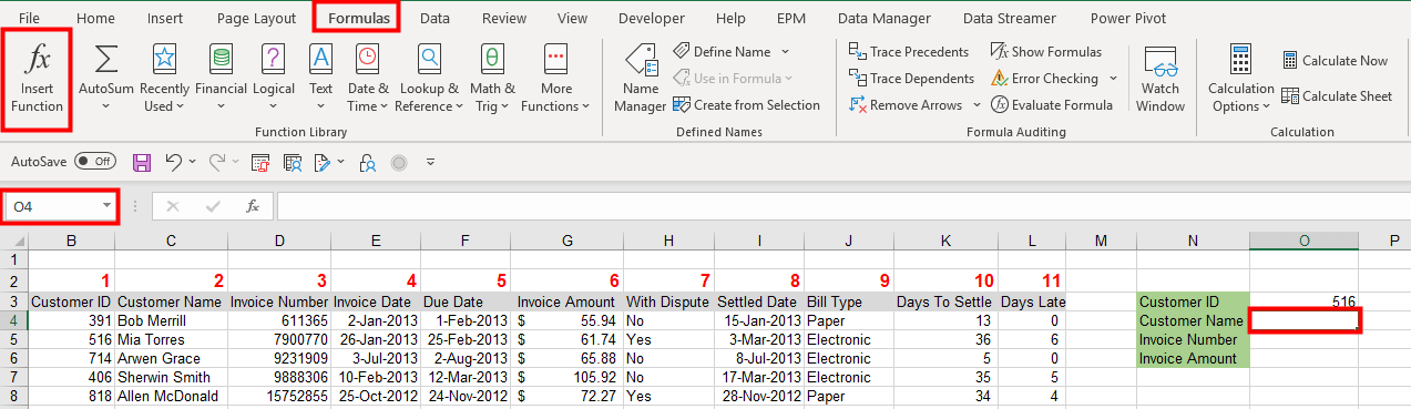
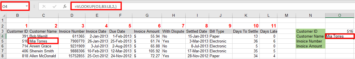
The purpose of the VLOOKUP function is to get data from a table that is organized vertically such as this:
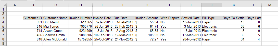
In the screen capture, the following data are available:
• Customer ID – column B
• Customer Name – column C
• Invoice Number – column D
• Invoice Date – column E
• Due Date – column F
• Invoice Amount – column G
• With Dispute – column H
• Settled Date – column I
• Bill Type – column J
• Days to Settle – column K
• Days Late – column L
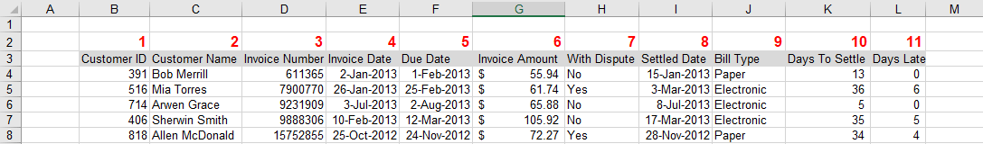
Note that the lookup value should be placed at the left side of the value you are looking for. Since the Customer ID is located in the leftmost column (column B), we can use it as a lookup value to get the corresponding Customer Name, Invoice Number, Invoice Date, Due Date, Disputed, Settled Date, Bill Type, Days to Settle and Days Late using the VLOOKUP function.
It is also important to remember that VLOOKUP is based on column numbers. When using this function, imagine that every column in the table array (data source) is numbered, starting from the left. To retrieve or return a value from a particular column, we should provide the “column index” in the syntax.
Using VLOOKUP Formula In Cell
If you opt to use the VLOOKUP function by typing the formula, go to the cell where you would like to display the result.
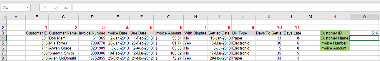
Using above data in the screen capture, let’s display the Customer Name of Customer ID 516 in cell O4.
Go to cell O4 and refer to the VLOOKUP syntax below:
=VLOOKUP(Lookup_Value, table_array, col_index_num,[range_lookup])
Simply, the syntax above means:
=VLOOKUP(What you want to look up, where you want to look for it, the column number in the range containing the value to return, return an Approximate or Exact match – indicated as 1/TRUE or 0/FALSE).
Now let’s identify the components:
1. Lookup_Value
a. Question: What you want to look up?
b. Answer: I want to look up the Customer Name for Customer ID located in cell O3.
2. Table_Array
a. Question: Where do you want to look for it?
b. Answer: I want to look at the data located in cells B3 to L8.
3. Col_Index_Num
a. Question: What is the column number in the range containing the value you want to return?
b. Answer: The column number for Customer Name which is the value I want to return is .
4. Range_Lookup (Optional)
a. Question: Would you like to return an approximate or exact match?
b. Answer: I want an exact match.
Now that we have identified the components of the syntax, we can now type the formula below:
O4 = VLOOKUP(O3, B3:L8,2,0)
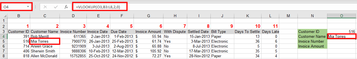
When you press enter after typing the above formula, cell O4 would display the corresponding Customer Name for Customer ID 516 which is Mia Torres.
Let’s try another example. Let’s look up the Invoice number of the Customer ID.
Again, identify the components:
1. Lookup_Value
a. Question: What you want to look up?
b. Answer: I want to look up the Invoice Number for Customer ID located in cell O3.
2. Table_Array
a. Question: Where do you want to look for it?
b. Answer: I want to look at the data located in cells B3 to L8.
3. Col_Index_Num
a. Question: What is the column number in the range containing the value you want to return?
b. Answer: The column number for Customer Name which is the value I want to return is 3
4. Range_Lookup (Optional)
a. Question: Would you like to return an approximate or exact match?
b. Answer: I want an exact match.
Now that we have identified the components of the syntax, we can now type the formula below:
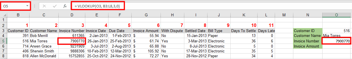
O5 = VLOOKUP(O3, B3:L8,3,0)

After clicking OK, cell O5 would display the corresponding Invoice Number for Customer ID 516 which is 7900770.
Using VLOOKUP Through INSERT MENU Option
Another way of using the VLOOKUP function is thru the Insert Function Menu. Place your cursor on the cell you want to display the result. In our example, that’s cell O4. Then click “Formulas” and select “Insert Function”.
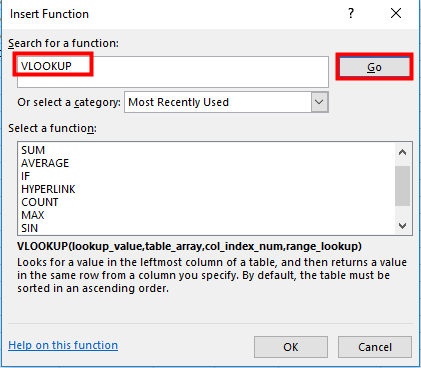
In the pop-up window, type “VLOOKUP” and click Go or press Enter.
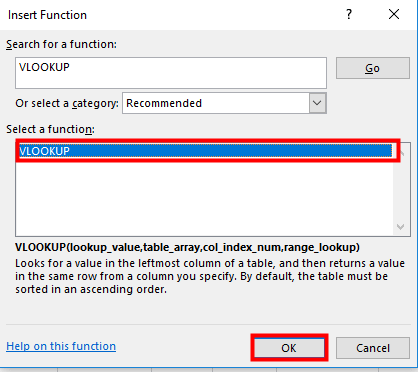
In the next pop-up window, ensure that the VLOOKUP function is highlighted. Click OK.
The next pop-up window will display the Function Arguments or the components of the syntax.
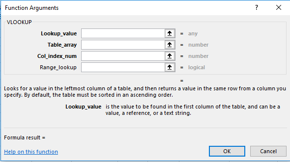
Using the guide listed in the earlier section of this article, fill out each argument. It should look like below screen capture. Then click OK.

Using the guide listed in the earlier section of this article, fill out each argument. It should look like below screen capture. Then click OK.
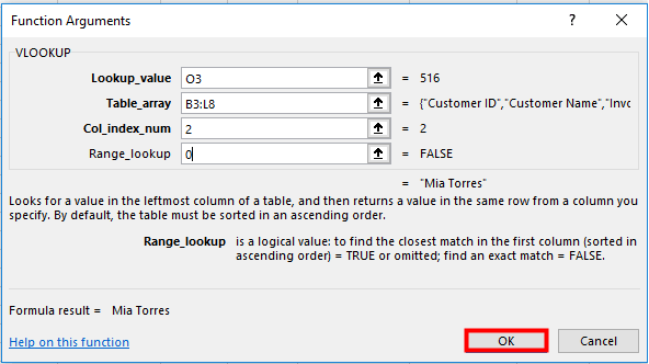
After clicking OK, cell O4 would display the corresponding Customer Name for Customer ID 516 which is Mia Torres.
Note that when you check the formula in cell O4 done thru the Insert Function menu, it is the same with the formula we used when typing the syntax.
Let’s try to return the Invoice number for Customer ID using the Insert Function feature.
To do this, place your cursor in cell O5 and repeat the steps above.
The difference would be this time, you should input “3” in Col_index_num Argument.
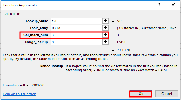
After clicking OK, cell O5 would display the corresponding Invoice Number for Customer ID 516 which is 7900770.
Note that when you check the formula in cell O5 done thru the Insert Function menu, it is the same with the formula we used when typing the syntax.
Related Notebooks
- How To Use Grep In R
- How To Use Python Pip
- How To Use Pandas Correlation Matrix
- How To Use R Dplyr Package
- How To Use Selenium Webdriver To Crawl Websites
- Return Multiple Values From a Function in Python
- What is LeakyReLU Activation Function
- Why do we use Optional ListNode in Python
- How To Write DataFrame To CSV In R
- Pandas group by multiple custom aggregate function on multiple columns