An Anatomy of Key Tricks in word2vec project with examples

import numpy as np
from collections import Counter
import mmap
import re
import networkx as nx
import math

MAX_EXP = 6
EXP_TABLE_SIZE = 1000
EXP_TABLE = np.arange(start = 0, stop = EXP_TABLE_SIZE, 
                      step = 1, dtype = np.float64)
## Exponentials of [-MAX_EXP, MAX_EXP]
EXP_TABLE = np.exp((EXP_TABLE / EXP_TABLE_SIZE * 2 - 1) * MAX_EXP)
## Logitstic Regression of [-MAX_EXP, MAX_EXP]
EXP_TABLE = EXP_TABLE / (EXP_TABLE + 1.)
## SO to use the EXP_TABLE, the value f must be in range [-MAX_EXP, MAX_EXP]
## and first transform the f value to range [0, EXP_TABLE-1]
## and then get the value from the table, e.g., to get logistic function value of f
f = [-6., -3., 0, 3., 6.]
## (f+MAX_EXP) / (MAX_EXP/2) transforms f to [0, 1]
index4exptable = lambda f: int((f+MAX_EXP) * (EXP_TABLE_SIZE/MAX_EXP/2))
f_index = map(index4exptable, f)
logistic_f = EXP_TABLE[f_index]
print f
print f_index
print logistic_f ## values in [0, 1] for logistic regression

class HashedVocab(object):
    HASH_SIZE = 30000000 ## max hash size
    ## count threshold for a word to be in the vocab - ignore infrequent word
    MIN_COUNT = 5 
    @staticmethod
    def file2ws(fpath):
        """
        file to wordstream: lazily read words from a file as an iterator
        """
        with open(fpath) as fin:
            word_pattern = re.compile(r'(.*?)\s')
            mf = mmap.mmap(fin.fileno(), 0, access = mmap.ACCESS_READ)
            for match in word_pattern.finditer(mf):
                word = match.group(1)
                if word: yield word
    def __init__(self):
        ## vocab stores vocab_word dict
        self.vocab = []
        ## vocab_hash stores the index of vocab_word in vocab
        self.vocab_hash = np.empty(HashedVocab.HASH_SIZE, dtype = np.int64)
        self.vocab_hash.fill(-1)
        ## house-keeping - total number of word occurences in training set
        ## it will be used as an estimate of training size later, which 
        ## affect the adjustment of learning rate of the deep structure
        self.n_train_words = 0
    def fit(self, word_stream):
        """
        build hashed_vocab and Huffman tree from word stream
        the word_stream is usually from reading a word file, e.g., using file2ws
        """
        ## word counter
        wc = Counter(word_stream)
        ## total occurances of training words
        self.n_train_words = sum(wc.values())
        ## Sort the words by their counts, filter out infrequent words,
        ## construct vocab_word (a dict) and put them in self.vocab
        self.vocab = map(lambda x: dict(zip(['word', 'count'], x)),
                         filter(lambda x: x[1] > HashedVocab.MIN_COUNT, 
                                wc.most_common(len(wc))))
        ## if vocab is already too big for hash, either (1) ignoring more infrequent
        ## words (as implemented in C by ReduceVocab), (2) making hash size bigger
        ## here we simply raise an exception for simplicity
        if len(self.vocab) > HashedVocab.HASH_SIZE * 0.7:
            raise RuntimeError('vocab size too large for hash, increase MIN_COUNT or HASH_SIZE')
        self.build_hash()
        self.build_huffman_tree()
        return self
    def index_of(self, word):
        """
        Get the index of word in vocab by using hash,
        return -1 if it is NOT there
        """
        word_hash = self.get_word_hash(word)
        while True:
            word_index = self.vocab_hash[word_hash]
            if word_index == -1:
                return -1
            elif word == self.vocab[word_index]['word']:
                return word_index
            else:
                word_hash = (word_hash + 1) % HashedVocab.HASH_SIZE
    def __getitem__(self, word_index):
        """
        get vocab_word in vocab by its index
        """
        return self.vocab[word_index]
    def __len__(self):
        return len(self.vocab)
    def __iter__(self):
        return iter(self.vocab)
    
    
    def build_hash(self):
        self.vocab_hash = np.empty(HashedVocab.HASH_SIZE, dtype = np.int64)
        self.vocab_hash.fill(-1)
        for word_index, vocab_word in enumerate(self.vocab):
            word = vocab_word['word']
            word_hash = self.get_word_hash(word)
            self.add_to_hash(word_hash, word_index)
        return self
    def get_word_hash(self, word):
        word_hash = sum([ord(c)*(257**i) 
                     for i, c in zip(range(len(word))[::-1], word)])
        word_hash %= HashedVocab.HASH_SIZE
        return word_hash
    def add_to_hash(self, word_hash, word_index):
        while self.vocab_hash[word_hash] != -1:
            word_hash = (word_hash + 1) % HashedVocab.HASH_SIZE
        self.vocab_hash[word_hash] = word_index
        return self
    def build_huffman_tree(self):
        """Build the Huffman tree representation for word based on their freq.
        The vocab_word structure in self.vocab is a dict {word, count, path, code}
        where vocab_word['code'] is the Huffman coding of word, and
        vocab_word['path'] will be the path from root to leaf
        """
        ## for a full binary tree with n leaves, n-1 internal nodes will be needed
        ## for the 2*n-1 long data array (e.g. count and binary), the first n will be
        ## for the leaf nodes, and the last n-1 will be for the internal nodes
        vocab_size = len(self)
        ## workhorse structure for tree construction
        ## count - the count of words (leaves) and internal nodes (sum of leave counts)
        count = np.empty(vocab_size * 2 - 1, dtype = np.int64)
        count.fill(1e15)
        count[:vocab_size] = [vw['count'] for vw in self.vocab]
        ## binary - boolean repr for leaves and internal nodes
        binary = np.zeros(vocab_size*2-1, dtype=np.int64)
        ## parent_node - storing the path for each node
        parent_node = np.empty(vocab_size*2-1, dtype = np.int64)
        ## construct the tree 
        ## DESCRIPTION: iteratively group the two ungrouped nodes (leaf or internal) that 
        ## have the smallest counts
        ## Since the vocab is sorted in decreasing counts order (first half ) and 
        ## the newly created internal nodes (second half) will be the order of 
        ## increasing counts (the algorithm invariant), so we only need to check
        ## the two nodes in the middle of array to look for candidates, that is the role
        ## of min1i and min2i
        ## start searching for min1i and min2i from the middle of array
        pos1, pos2 = vocab_size - 1, vocab_size
        ## construct the vocab_size -1 internal nodes
        for a in xrange(vocab_size-1):
            ## min1i
            if pos1 >= 0:
                # min1i = pos1
                if count[pos1] < count[pos2]:
                    min1i, pos1 = pos1, pos1-1
                # min1i = pos2
                else: 
                    min1i, pos2 = pos2, pos2+1
            else: ## running out of leaf nodes
                min1i, pos2 = pos2, pos2+1
            ## min2i
            if pos1 >= 0:
                if count[pos1] < count[pos2]:
                    min2i, pos1 = pos1, pos1-1
                else:
                    min2i, pos2 = pos2, pos2+1
            else:
                min2i, pos2 = pos2, pos2+1
            ## count(parent_node) = count(child1) + count(child2)
            count[vocab_size + a] = count[min1i] + count[min2i]
            ## link parent node index
            parent_node[min1i] = vocab_size + a
            parent_node[min2i] = vocab_size + a
            ## binary encoding for min1i is 0 (left), for min2i is 1 (right)
            binary[min2i] = 1
        ## put the built Huffman tree structure in the vocab_word in vocab
        ## for each leaf node
        for a in xrange(vocab_size):
            ## b starting from leaf, along parent_nodes, to the root
            b = a
            code, path = [], []
            ## traverse along the path to root
            while True:
                code.append(binary[b])
                path.append(b)
                b = parent_node[b]
                ## stop when reaching root
                if b == vocab_size * 2 - 2: break
            ## path (or point) is from root to leaf, with an index offset
            ## -vocab_size
            self.vocab[a]['path'] = [vocab_size - 2] + [p - vocab_size
                                                        for p in path[::-1]]
            self.vocab[a]['code'] = code[::-1]
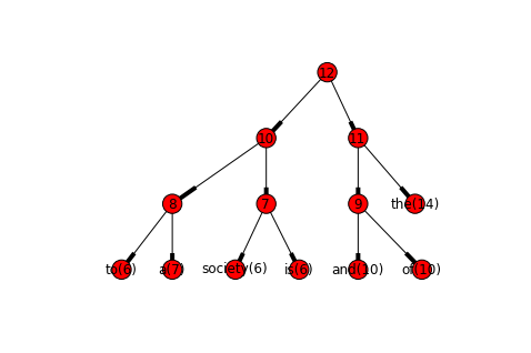
    def inspect_vocab_tree(self):
        """Draw the built Huffman binary tree for the vocab
        """
        g = nx.DiGraph()
        vocab_size = len(self)
        edges = set()
        for vw in self.vocab:
            tree_path = [i + vocab_size for i in vw['path']]
            tree_path = [i if i >= vocab_size
                         else "%s(%d)" % (self.vocab[i]['word'], self.vocab[i]['count'])
                         for i in tree_path]
            edges.update(zip(tree_path[:-1], tree_path[1:]))
        g.add_edges_from(edges)
        pos = nx.graphviz_layout(g, prog = 'dot')
        nx.draw(g, pos, with_labels = True, arrows = True)
        return g

## examples of buiding the hashed_vocab and its associated Huffman tree
## simple.txt is the first 50K words from original text8
hashed_vocab = HashedVocab()
hashed_vocab.fit(HashedVocab.file2ws('data/first50k.txt'))
print 'totally %i words were used to build vocab' % hashed_vocab.n_train_words
print '%i of them go into the vocab' % len(hashed_vocab)

## simple example to illustrate the built Huffman tree
%pylab inline
hashed_vocab = HashedVocab().fit(HashedVocab.file2ws('data/first300.txt'))
hashed_vocab.inspect_vocab_tree()

class UnigramTable(object):
    TABLE_SIZE = int(1e8)
    POWER = 0.75
    def __init__(self, hashed_vocab):
        self.table = np.empty(UnigramTable.TABLE_SIZE, np.int64)
        vocab = hashed_vocab
        vocab_size = len(hashed_vocab)
        ## normalization factor of all word's frequency's power
        train_words_pow = sum(math.pow(vw['count'], UnigramTable.POWER)
                              for vw in vocab)
        ## doing the sampling in the table
        ## the sampling probability of a unigram is proportional to its
        ## frequency to a power of POWER (=0.75)
        
        ## i marks the index of current word in vocab
        ## d1 marks the accumulative power-law probability up to the current word
        ## a / TABLE_SIZE marks the sampling proability up to the current word
        i = 0
        d1 = math.pow(vocab[i]['count'], UnigramTable.POWER) / train_words_pow
        for a in xrange(self.TABLE_SIZE):
            self.table[a] = i
            ## compare accumulative sampling prob with power-law accumulative prob
            ## move to the sampling of next word if they start not matching
            if a * 1. / UnigramTable.TABLE_SIZE > d1:
                i += 1
                d1 += math.pow(vocab[i]['count'], UnigramTable.POWER) / train_words_pow
            ## put the rest as sampling of the last word (round-off)
            if i >= vocab_size:
                i = vocab_size - 1
    def __getitem__(self, index):
        return self.table[index]

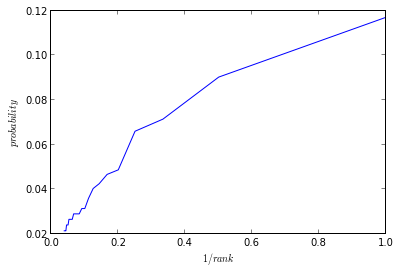
## check how satisfying the sampling strategy is to the Zipf's law
## http://mathworld.wolfram.com/ZipfsLaw.html
hashed_vocab = HashedVocab().fit(HashedVocab.file2ws('data/first1k.txt'))
unigram_table = UnigramTable(hashed_vocab)
sampling_probs = [sum(unigram_table.table == i) / 1e8 for i in xrange(len(hashed_vocab))]
plot(1./np.arange(1, len(hashed_vocab)+1), sampling_probs)
xlabel('$1/rank$')
ylabel('$probability$')

class CBOW(object):
    REAL_TYPE = np.float64
    def __init__(self, hashed_vocab, unigram_table,
                 layer1_size, learn_hs, learn_negative):
        """
        hashed_vocab: the vocab to build on
        layer1_size: the size of layer1 of the net, effectively defines the dim of feature space
        learn_hs: use hierarchical softmax learning
        learn_negative: use negative sampling learning
        """
        self.vocab = hashed_vocab
        self.table = unigram_table
        self.layer1_size = layer1_size
        self.learn_hs = learn_hs
        self.learn_negative = learn_negative
        
        ## initial value for learning rate, will decrease along learning
        self.starting_alpha = 0.025
        ## a sentence is a bulk of words from train file
        self.sentence_len = 1000
        ## downsampling rate to select words into a sentence
        self.sampling = 1e-4
        ## window defines the neighborhood of a word in the sentence for hs learning
        self.window = 5
        ## negative defines the neighborhood of a word for negative learning
        self.negative = 5
        
        ## network weights
        ## syn0 - feature representations of words (leaf nodes) in Huffman tree
        ## shape = vocab_size x layer1_size
        self.syn0 = None 
        ## syn1 - feature representations of internal nodes (non-leaf) in Huffman tree
        ## shape = vocab_size x layer1_size
        self.syn1 = None ## hidden layer for hs learning
        ## syn1neg - feature representations of negative-sampled words
        ## shape = vocab_size x layer1_size
        self.syn1neg = None ## hidden layer for negative learning
    def init_net(self):
        """
        """
        vocab_size = len(self.vocab)
        self.syn0 = np.random.uniform(low = -.5 / self.layer1_size, 
                                      high = .5 / self.layer1_size,
                                      size = (vocab_size, self.layer1_size)).astype(CBOW.REAL_TYPE)
        if self.learn_hs:
            self.syn1 = np.zeros((vocab_size, self.layer1_size), dtype=CBOW.REAL_TYPE)
        if self.learn_negative:
            self.syn1neg = np.zeros((vocab_size, self.layer1_size), dtype = CBOW.REAL_TYPE)
    def fit(self, train_words):
        """
        train_words: list of training words
        """
        ## initialize net structure
        self.init_net()
        ntotal = len(train_words)
        ## initialize learning parameters
        alpha = self.starting_alpha
        next_random = 0
        
        ## read and process words sentence by sentence
        ## from the train_words 
        nprocessed = 0
        while nprocessed < ntotal:
            ## adjust learning rate based on how many words have
            ## been trained on
            alpha = max(self.starting_alpha * (1-nprocessed/(ntotal+1.)),
                        self.starting_alpha * 0.0001)
            ## refill the sentence
            sentence = []
            while nprocessed < ntotal and len(sentence) < self.sentence_len:
                ## sampling down the infrequent words
                word = train_words[nprocessed]
                word_index = self.vocab.index_of(word)
                nprocessed += 1
                if word_index == -1: continue
                word_count = self.vocab[word_index]['count']
                if self.sampling > 0:
                    ran = ( (math.sqrt(word_count / (self.sampling * ntotal)) + 1) 
                            * (self.sampling * ntotal) / word_count )
                    next_random = next_random * 25214903917 + 11
                    ## down sampling based on word frequency
                    if ran < (next_random & 0xFFFF) / 65536: continue
                sentence.append(word_index)
            ## for each word in the preloaded sentence
            ## pivot is the vocab index of current word to be trained on
            ## ipivot is the index in the current setence
            for ipivot, pivot in enumerate(sentence):
                next_random = next_random * 25214903917 + 11
                ## window-b defines the length of the window
                ## which is the neighborhood size for the current
                ## word in the sentence
                b = next_random % self.window
                ## initialize temp variable
                ## neu1: the sum of neigbhor vectors in the setence
                ## neu1e: the gradient vector wrt syn0
                ## see the explaination above the code
                neu1 = np.zeros(self.layer1_size, dtype = self.REAL_TYPE)
                neu1e = np.zeros(self.layer1_size, dtype = self.REAL_TYPE)
                ## accumulate sum of neighbor words into neu1
                ## neighbors are defined as [ipivot-(window-b), ipivot+(window-b)]
                left = max(0, ipivot - (self.window-b))
                right = min(len(sentence)-1, ipivot+self.window-b)
                ## all neighborhood index should >= 0 (in vocab) as otherwise
                ## it won't go into the sentence in the first place
                neighborhood = [sentence[n] for n in range(left, right+1) 
                                    if sentence[n] >= 0]
                neu1 = np.sum(self.syn0[neighborhood,:], axis = 0)
                ## hierarchical softmax learning
                if self.learn_hs:
                    ## for each output node in layer1 
                    ## which are parent nodes of pivot in Huffman tree
                    ## notice the last element of 'path' is the word itself, 
                    ## so exclude it here 
                    for parent_index, parent_code in zip(self.vocab[pivot]['path'][:-1],
                                                             self.vocab[pivot]['code']):
                        ## F is the logistic transformation of dot product 
                        ## between neu1 and each parent repr in syn1
                        f = np.dot(neu1, self.syn1[parent_index, :])
                        ## output out of range
                        if f <= - MAX_EXP or f >= MAX_EXP:
                            continue
                        ## logistic function transformation
                        else:
                            f = EXP_TABLE[int((f + MAX_EXP) * (EXP_TABLE_SIZE / MAX_EXP / 2))]
                        ## pseduo target is 1 - parent_code
                        g = (1 - parent_code - f) * alpha
                        ## accumulate neu1 to update syn0 later
                        neu1e += g * self.syn1[parent_index]
                        ## update syn1 of current parent
                        self.syn1[parent_index] += g * neu1
                ## negative sampling learning
                ## select one positive and several negative samples
                if self.learn_negative:
                    for d in range(self.negative + 1):
                        ## make sure to select the current word
                        ## as positive sample
                        if d == 0:
                            target = pivot
                            label = 1
                        ## select some 'negative' samples randomly
                        else:
                            next_random = next_random * 25214903917 + 11
                            target = self.table[(next_random >> 16) % self.table.TABLE_SIZE]
                            if (target == pivot): continue ## ignore if it is still positive
                            label = 0
                        ## this time f is dot product of neu1 with 
                        ## syn1neg
                        f = np.dot(neu1, self.syn1neg[target, :])
                        ## pseudo target is label
                        ## NOTE the differece between hs and negative-sampling
                        ## when dealing with f out of [-MAX_EXP, MAX_EXP]
                        if f > MAX_EXP:
                            g = (label - 1) * alpha 
                        elif f < - MAX_EXP:
                            g = (label - 0) * alpha
                        else:
                            g = alpha * (label - 
                                    EXP_TABLE[int((f + MAX_EXP) 
                                        * (EXP_TABLE_SIZE / MAX_EXP / 2))])
                        ## accumulate changes to syn0 to neu1e again
                        neu1e += g * self.syn1neg[target]
                ## update syn0 after hs and/or negative-sampling learning
                self.syn0[neighborhood, :] += neu1e

## test cbow
hashed_vocab = HashedVocab().fit(HashedVocab.file2ws('data/first50k.txt'))
unigram_table = UnigramTable(hashed_vocab)
train_words = list(HashedVocab.file2ws('data/first50k.txt'))

cbow_model = CBOW(hashed_vocab, unigram_table,
                  layer1_size = 50, 
                  learn_hs = True, learn_negative = True)
cbow_model.fit(train_words)

from numpy import linalg
Xnorm = np.apply_along_axis(linalg.norm, 1, cbow_model.syn0)
#X = cbow_model.syn0 / Xnorm[:, np.newaxis]
X = cbow_model.syn0
word = cbow_model.vocab.index_of('one')
word_vec = X[word]
#closest_words = np.dot(X, guess).argsort()[::-1]
closest_words = np.sum((X - word_vec)**2, axis = 1).argsort()
for i in closest_words[:5]:
    print cbow_model.vocab[i]['word']