This tutorial shows a full use-case of PyTorch in order to explain several concepts by example. The application will be hand-written number detection using MNIST. MNIST is a popular (perhaps the most popular) educational computer vision dataset. It is composed of 70K images of hand-written digits (0-9) split into 60K-10K training and test sets respectively. The images are tiny (28x28), which makes them easy to work with.
PyTorch Data Loading
When using PyTorch, there are many ways to load your data. It depends mainly on the type of data (tables, images, text, audio, etc.) and the size. Many text datasets are small enough to load into memory in full. Some image datasets (such as MNIST can also be loaded to memory in full due to the small image size. However, in most real-life applications, the datasets will be too large to load into memory in full.
The way PyTorch handles this problem is simple: datasets, data loaders and batch iterators.
A Dataset in PyTorch contains all the data. When we initialize a dataset in PyTorch, we can also specify certain transformations to apply.
Data Loaders receive dataset objects as input and create a blueprint of batches.
Batch Iterators: Batch iterators loop over the data in batches (of 16, 32, for example) provided by the data loader. Then, a full training loop is performed on this subset. Once finished, the current batch is discarded and a new batch is loaded for training.
By using these above concepts, PyTorch is able to perform preprocessing, transformations, and training on small batches of data without running out of memory.
Let us start by importing the required libraries and tools:
import os
import random
import numpy as np
import pandas as pd
from PIL import Image
from sklearn.metrics import accuracy_score
import torch
from torch import nn
import torch.nn.functional as F
from torch.utils.data import Dataset, DataLoader
from torchvision import datasets
from torchvision.transforms import ToTensor
import matplotlib.pyplot as plt
Not that torch.utils.data.Dataset is the dataset class we can extend, whereas torchvision.datasets are just a group of ready to use datasets (such as MNIST) in the PyTorch library.
Since MNIST is already provided as a ready dataset, we just need to download the training and test sets as follows:
training_ds = datasets.MNIST(
    root="data",
    train=True,
    download=True,
    transform=ToTensor(), # A quick way to convert the image from PIL image to tensor
)

test_ds = datasets.MNIST(
    root="data",
    train=False,
    download=True,
    transform=ToTensor(),
)
The dataset which is stored locally, you can create it as follows:
class LocalDS(Dataset):
    def __init__(self, data_dir, label_dir, root_dir, transforms):

        self.data_dir = data_dir
        self.label_dir = label_dir
        self.root_dir = root_dir
        self.transforms = transforms

        #Creating path lists
        self.img_paths = os.path.join(self.root_dir, self.data_dir)
        self.label_paths = os.path.join(self.root_dir, self.label_dir)

    def __len__(self):
        return len(self.img_paths)

    def __getitem__(self, idx):
        """
            This is the critical method in this class. It allows us to get
            an instance by an id.
        """
        img = Image.open(self.img_paths[idx])
        label = label_paths[idx]

        if self.transforms:
            img = self.transforms(img)

        return img, label
This is a pseudocode example. You should modify it according to the structure of your dataset. But the key ideas are: image paths and labels are stored, and a __getitem__() method returns an image and its label. The __len__() method is optional but useful.
Let's test training_ds and test_ds to make sure they operate as we expect:
print(f"Size of training set: {len(training_ds)} images.")
print(f"Size of training set: {len(test_ds)} images.")
img, lbl = training_ds[0]
print(f"Image dimensions: {img.shape}.")
print(f"Image label: {lbl}.")
As we can see, len(training_ds) returns the number of paths (or images) in the dataset.
And, training_ds[0] returns the first image and its label.
So far, so good.
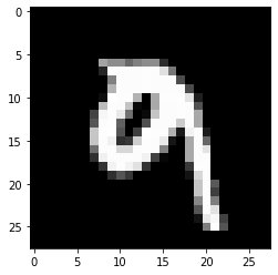
Now, let's visualize a random image.
The image dimensions are 1x28x28. To visualize the image, we must have it in 2D space, or simply 28x28. To remove a dimension from a tensor, use squeeze(). Similarly, to add a dimension, use unsqueeze(). Read the docs for more examples: https://pytorch.org/docs/stable/generated/torch.squeeze.html
random_id = random.randint(0, len(training_ds))
img, lbl = training_ds[random_id]
img.squeeze().shape
plt.imshow(img.squeeze(), cmap="gray")
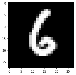
lbl
Great. Next are the dataloaders. Creating dataloaders in PyTorch is easy:
train_dataloader = DataLoader(training_ds, batch_size=128, shuffle=True)
test_dataloader = DataLoader(test_ds, batch_size=128, shuffle=True)
shuffle = True means that the dataset will be shuffled before being split into batches. This randomizes the batches which is good for generalization.
Using torch.nn, one can create any kind of model. In this tutorial, we explore the skeleton and guidelines to follow when creating a NN and in the process create a simple feed-forward NN (FFNN).
A NN in PyTorch is a class extending from nn.Module with __init__() and forward() methods. Of course we can add more methods, but these are the key components.
In __init__(), we create the architecture (the layers). A FFNN is composed of several fully-connected layers. Fully-connected layers are created using nn.Linear().
nn.Linear() takes in 2 arguments: number of inputs and number of outputs. When connecting FCs, you must make sure of 3 things:
- The number of inputs in the first layer must match the size of the data.
- The number of outputs of every layer must match the number of inputs in the next layer.
- The number of outputs in the final layer must match the number of classes you are working with.
Since FFNNs expect input as a vector (not a 2D tensor such as images), we cannot simply feed in the 28x28 vectors of MNIST images. We must flatten them into a 28*28 = 784 vector.
In advanced CV projects, the images will be larger than 28x28, and this approach will be unviable. For advanced CV applications, the CNN is a common architecture to use.
forward() takes in a batch and returns predictions for each class for each instance. In the forward() function, we manually pass the data from each layer to the next until the final layer.
class FFNN(nn.Module): # Extending nn.Module allows us to create NNs
    def __init__(self):
        super(FFNN, self).__init__()
        self.fc1 = nn.Linear(28*28, 128)  # Input is 28*28 = 784, output is 128 (can be anything)
        self.fc2 = nn.Linear(128, 512)    # Input is 128 since output of fc1 is 128
        self.fc3 = nn.Linear(512, 128)    # Input is 512 since output of fc2 is 512
        self.fc4 = nn.Linear(128, 10)     # Input is 128 since output of fc3 is 128,
                                          #   and output is 10 since there are 10 classes

    def forward(self, x):
        x = x.view(x.size(0), -1)         # Flattening
        x = F.relu(self.fc1(x))           # We feed the flattened images to to fc1 and perform ReLU
        x = F.relu(self.fc2(x))           # We do the same for all FC layers
        x = F.relu(self.fc3(x))
        logits = self.fc4(x)              # Finally, we get the predictions from fc4 or the output layer
        return logits
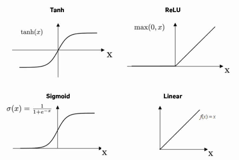
F.relu() is a popular activation function used after FC layers. Other alternatives are `F.tanh()` and `F.sigmoid()`, but ReLu has been shown to perform better.
To initialize and use the model, let us first set the device:
device = torch.device("cuda" if torch.cuda.is_available() else "cpu")
device
model = FFNN()
model = model.to(device)
model
Great. The data is ready and the model is ready. All that is left is the training.
Loss Functions and Optimizers
So far, we have prepared the data and the model. But, to train our model, we must perform some sort of gradient descent optimization in order to improve the model. To do so, we have to define a measure of quality. This measure is called the loss function, and it depends on the task. If the task is regression, loss functions such as MSE or RMSE can be used. For multi-label classification such as in MNIST, a common loss function is the cross-entropy loss. In short, it measures the quality of a prediction. Using this measure, we can optimize the loss of the model (reduce the error) iteratively using an optimizer. There are many optimizers proposed by the literature. The classic approach is to use Stochastic Gradient Descent (SGD), but a more popular optimizer is Adam. A lit of all optimizers in PyTorch can be found at https://pytorch.org/docs/stable/optim.html.
Let's create our loss function and optimizer:
criterion = nn.CrossEntropyLoss()
optim = torch.optim.Adam(model.parameters(), lr = 1e-3)
As shown, optimizers typically take 2 arguments: the model weights to optimize, and the learning rate. Here, we select a learning rate of 0.003, but other values are also acceptable. However, a really large learning rate may cause the model to never converge, and a very small learning rate my take too long. LRs in the range of 0.001 to 0.0003 are acceptable in most cases. There are more advanced solutions to adaptively change the LR during training.
Training is done in epochs. An epoch is simply 1 iteration over all the training data, typically followed by an iteration over the test data. In each epoch, we iterate over the data in batches. The general skeleton of a training epoch is as follows:
def run_epoch(loader, model, optimizer, criterion):
    for batch in loader:
        imgs, lbls = batch
        optimizer.zero_grad()
        with torch.set_grad_enabled(True): #Or False if testing
            logits = model(imgs)
            loss = criterion(logits, lbls)
            loss.backward()
            optimizer.step()
There are several things to explain in this block:
optimizer.zero_grad()with torch.set_grad_enabled()loss.backward()optimizer.step()optimizer.zero_grad()resets the optimizer gradients to zero. This is necessary before each batch so that backpropagation is optimizing only for current batch.with torch.set_grad_enabled()determines whether or not to calculate gradients (i.e. calculate performance). This method takes 1 argument: True or False, depending on wheter or not you are doing training/testing. In the test loop, this must be set to False to avoid training on the test set.loss.backward()andoptimizer.step()perform backpropagation on the current gradients and update the weights of the model to improve it.
Notice that we never call model.forward() explicitly. The forward function is simply called explicitly by model().
Finally, since this is the loop for one epoch, we can train on more epoch simply by doing this:
def main(epochs):
    for epoch in range(epochs):
        run_epoch()
Using these two functions, we can perform training and testing easily:
def run_epoch(ep_id, action, loader, model, optimizer, criterion):
    accuracies = [] # Keep list of accuracies to track progress
    is_training = action == "train" # True when action == "train", else False

    # Looping over all batches
    for batch_idx, batch in enumerate(loader):
            imgs, lbls = batch

            # Sending images and labels to device
            imgs = imgs.to(device)
            lbls = lbls.to(device)

            # Resetting the optimizer gradients
            optimizer.zero_grad()

            # Setting model to train or test
            with torch.set_grad_enabled(is_training):

                # Feed batch to model
                logits = model(imgs)

                # Calculate the loss based on predictions and real labels
                loss = criterion(logits, lbls)

                # Using torch.max() to get the highest prediction
                _, preds = torch.max(logits, 1)

                # Calculating accuracy between real labels and predicted labels
                # Notice that tensors must be on CPU to perform such calculations
                acc = accuracy_score(preds.to('cpu'), lbls.to('cpu'))

                # If training, perform backprop and update weights
                if is_training:
                    loss.backward()
                    optimizer.step()

                # Append current batch accuracy
                accuracies.append(acc)

                # Print some stats every 50th batch
                if batch_idx % 50 == 0:
                    print(f"{action.capitalize()}ing, Epoch: {ep_id+1}, Batch {batch_idx}: Loss = {loss.item()}, Acc = {acc}")
    # Return accuracies to main loop
    return accuracies
def main(epochs, train_dl, test_dl, model, optimizer, criterion):

    # Keep lists of accuracies to track performance on train and test sets
    train_accuracies = []
    test_accuracies = []

    # Looping over epochs
    for epoch in range(epochs):

        # Looping over train set and training
        train_acc = run_epoch(epoch, "train", train_dl, model, optimizer, criterion)

        # Looping over test set
        test_acc = run_epoch(epoch, "test", test_dl, model, optimizer, criterion)

        # Collecting stats
        train_accuracies += train_acc
        test_accuracies += test_acc

    return train_accuracies, test_accuracies
train_accs, test_accs = main(3, train_dataloader, test_dataloader, model, optim, criterion)
As shown by the accuracy scores, the model quickly learns to classify the images. At the end of training, the test accuarcy is ~98%, which is great.
We can visualize the progress of training by plotting the collected accuacies:
plt.plot(train_accs)
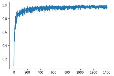
plt.plot(test_accs)
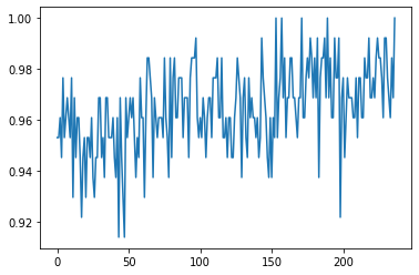
In both plots, the accuracy is very good near the end of training.
In classification, accuracy is only 1 metric. In real life applications, we must make sure that the data is balanced and to report recall, precision, and f1-score. These metrics can be found on the sklearn metrics module and they are used the same way we used accuracy_score()
Now, let us test the model to make sure it is actually functioning.
# Get a random test image
random_id = random.randint(0, len(test_ds))
img, lbl = training_ds[random_id]
plt.imshow(img.squeeze(), cmap="gray")
lbl
# First, send the image to device
img = img.to(device)
# Feed the image to the model
logits = model(img)
# Get the class with the highest score
_, preds = torch.max(logits, 1)
pred = preds.item()
pred
pred == lbl
As shown, in almost all random test cases, the model is capable of predicting the correct class.
Now that we have a trained model, we should save it to disk. That way, we can quickly load it whenever we need predictions without having to train the model again. Saving and loading models is very simple in PyTorch:
# Saving current weights:
path = "mnist_model.pt"
torch.save(model.state_dict(), path)
Now, let's initialize a new model without loading the weights:
new_model = FFNN()
new_model = new_model.to(device)
Since this model is untrained, we expect it to perform poorly when predicting:
logits = new_model(img)
_, preds = torch.max(logits, 1)
pred = preds.item()
pred
pred == lbl
As expected, it does not perform well.
Now, let's load the trained weights from disk:
new_model.load_state_dict(torch.load(path))
Finally, let's make sure that the new model performs properly:
logits = new_model(img)
_, preds = torch.max(logits, 1)
pred = preds.item()
pred
pred == lbl
Great! Now we can train models and save them for later use quickly.