Activation Functions In Artificial Neural Networks Part 2 Binary Classification
This is part 2 of the series on activation functions in artificial neural networks. Chek out part1 - how to use RELU in Artificial Neural Networks for building a Regression model.
In this notebook, I will talk about how to build a binary classification neural network model.
from collections import Counter

import matplotlib.pyplot as plt
import numpy as np
import pandas as pd
import tensorflow as tf
from sklearn.datasets import load_boston
from sklearn.model_selection import train_test_split
from tensorflow.keras.layers import Dense, Dropout, Input
from tensorflow.keras.models import Model
To ensure that every time we run the code we get the same results, we need following code so as to generate a fixed random seed.
tf.random.set_seed(42)
np.random.seed(42)
For this exercise, we will use breast cancer dataset which is available in sklearn datasets.
from sklearn.metrics import classification_report
from sklearn.datasets import load_breast_cancer
data = load_breast_cancer()
X = data["data"]
y = data["target"]
labels = data["target_names"]
X_train, X_test, y_train, y_test= train_test_split(X, y, random_state=42)
def annotate_bars(ax, patches, horizontal=False, as_int=True):
    for p in patches:
        if horizontal:
            w = p.get_width()
            w = int(w) if as_int else round(w, 3)
            if w == 0:
                continue
            ax.annotate(f"{w}", (p.get_width()* 1.01, p.get_y() +0.1), fontsize=14)
        else:
            h = p.get_height()
            h = int(h) if as_int else round(h, 3)
            if h == 0:
                continue
            ax.annotate(f"{h}", (p.get_x() +p.get_width()/2, p.get_height()* 1.01), fontsize=14)
    return ax
counter = Counter(y)
keys = counter.keys()
values = counter.values()
fig = plt.figure(figsize=(16, 9))
bar = plt.bar(keys, values)
annotate_bars(plt, bar.patches)
plt.xticks([0, 1], labels=["malignant", "benign"])
plt.xlabel("Class", fontsize=16)
plt.ylabel("Frequency", fontsize=16)
plt.title("Labels Distribution", fontsize=22)
plt.show()
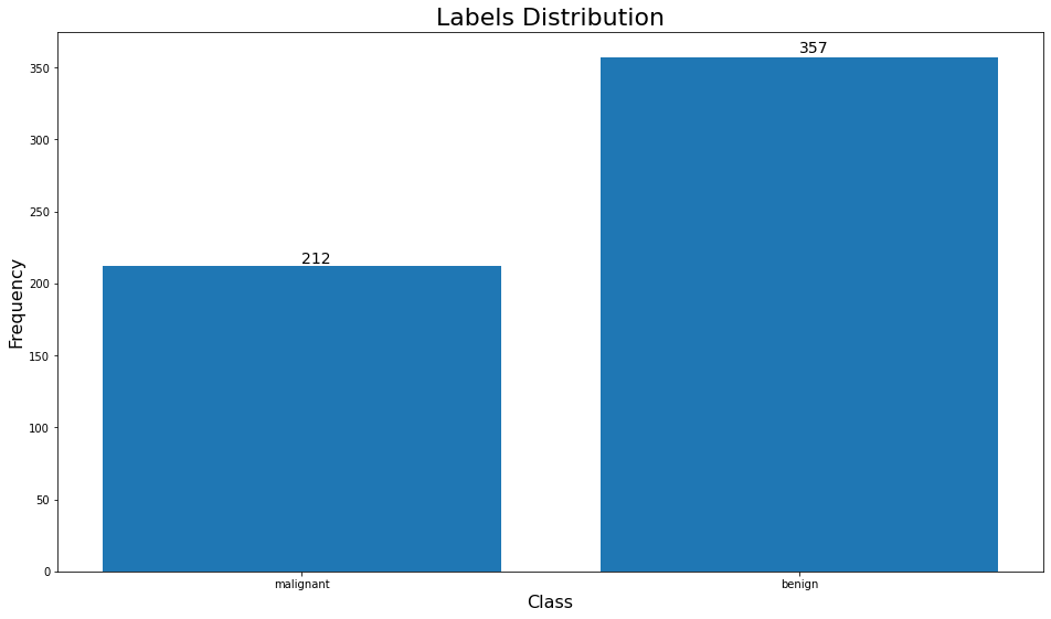
We notice that the data is imbalanced, so we will need to do something about that before we train our model.
from sklearn.utils import compute_class_weight
class_weight = compute_class_weight('balanced', [0, 1], y_train)
class_weight
class_weight_dict = dict(zip([0, 1], class_weight))
class_weight_dict
In the above code, we are giving higher weight to the under represented class 0 (i.e. malignant)
input_shape = X.shape[1] # number of features, which is 30
This is binary classification, So we only need one neuron to represent the probability of classifying the sample with the positive label.
output_shape = 1
Since this is a binary classification problem, we want the output to represent the probability of the selecting the positive class. In other words, we want the output to be between 0 and 1. A typical activation function for this is the *sigmoid* function. The sigmoid function is an example of the logistic function we use in logistic regression. It is an S-shaped curve that squashes the values to be between 0 and 1.
inputs = Input(shape=(input_shape,))
h = Dense(32, activation="relu")(inputs)
h = Dense(16, activation="relu")(h)
h = Dense(8, activation="relu")(h)
h = Dense(4, activation="relu")(h)
out = Dense(output_shape, activation="sigmoid")(h)
model = Model(inputs=inputs, outputs=[out])
model.summary()
We use binarycrossentropy as the loss we want to minimize. This is the same one we have seen in logistic regression. $$-\frac{1}{n}\sum{i=1}^N{y_i\log(\hat{y_i})+(1-y_i)\log(1-\hat{y_i})}$$
model.compile(optimizer="adam", loss="binary_crossentropy", metrics="accuracy")
H = model.fit(
    x=X_train,
    y=y_train,
    validation_data=(
        X_test, y_test
    ),
    class_weight=class_weight_dict,
    epochs=50,
)
f, axarr = plt.subplots(1,2, figsize=(16, 9))
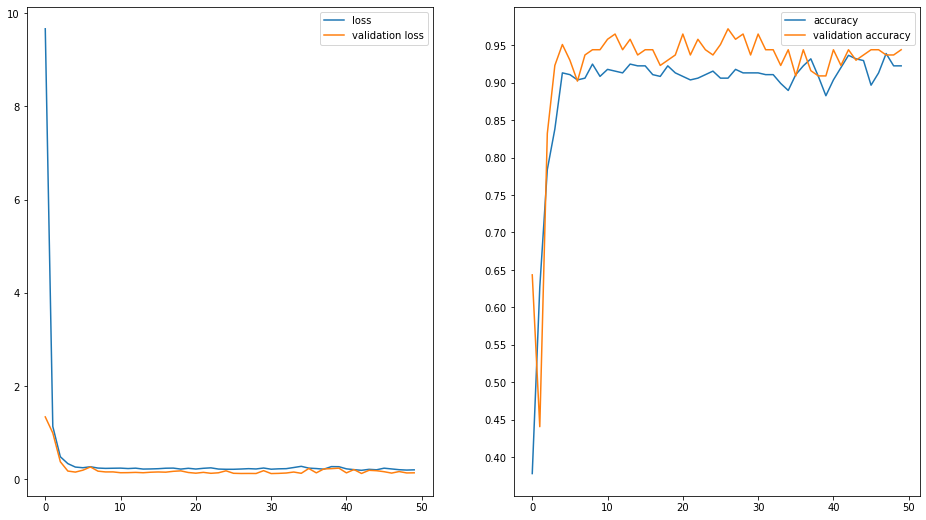
axarr[0].plot(H.history["loss"], label="loss")
axarr[0].plot(H.history["val_loss"], label="validation loss")
axarr[0].legend()
axarr[1].plot(H.history["accuracy"], label="accuracy")
axarr[1].plot(H.history["val_accuracy"], label="validation accuracy")
axarr[1].legend()
axarr[1].set_yticks(np.arange(0.4, 1, 0.05))
plt.show()
Let us now predict the probabilities.
pred_probs = model.predict(X_test) # predicted probabilities
y_pred=  pred_probs>=0.5 # higher than 50% probability means a positive class (i.e. class 1 or malignant)
print(classification_report(y_test, y_pred))
Related Notebooks
- Rectified Linear Unit For Artificial Neural Networks Part 1 Regression
- How To Code RNN and LSTM Neural Networks in Python
- Activation Functions In Python
- Generative Adversarial Networks
- Best Approach To Map Enums to Functions in Python
- Movie Name Generation Using GPT-2
- Amazon Review Summarization Using GPT-2 And PyTorch
- Boxplots In R
- Append In Python