Pivot Tables In Excel
Pivot tables in excel is one of the most important utility to do data analysis. In this tutorial I will go over step by step of how to make pivot tables in excel.
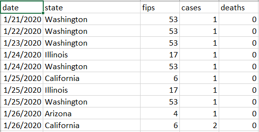
For this exercise, I have downloaded a CSV file (shown below) which has US corona virus cases by state and date. The CSV file can be downloaded from here...
https://github.com/nytimes/covid-19-data
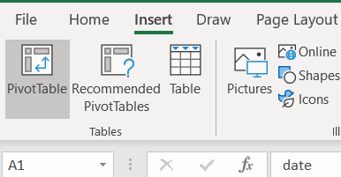
To draw the pivot table, click "Pivot Table" under the "insert" tab as shown below.
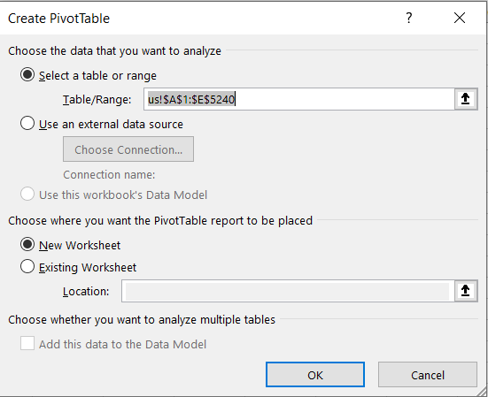
After you do the above step, A dialog box will open up as show below for "Create PivotTable". In the below snapshot, note "Table/Range" field and its values. By default Pivot table will be created for all the values in the table from A1:E5240. We can change these values here in this field if we want to create the pivot table for partial data. But for now we will keep the default values for our pivot table. Leave all the settings as it is and click ok. A new sheet will be created for the pivot table by Excel.
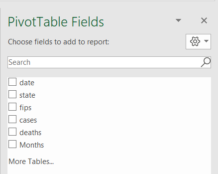
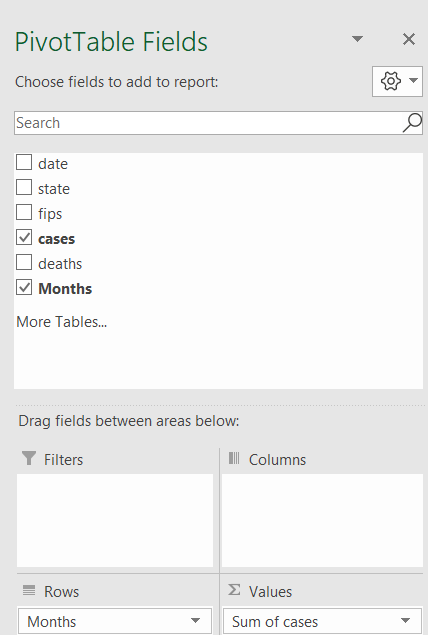
In the new sheet, you will see the Pivot Table Fields on the right hand side as shown below. As seen in the blow snapshot, all the headers from the table are copied which we can select to build our Pivot table. Note: There is extra field "Months" added by Excel that is derived from date field in the list of headers to choose from.
There are multiple ways to build the pivot table and it depends upon which fields we chose for columns,rows, filter and values.
To build these tables, easy way is to think like how do we want to visualize or analyze our data or what information we want to extract out.
Example: Problem statement: Show me the total number of cases by each month in USA.
To solve the above problem, we need to group the data by month. Therefore that means month will go to rows. Since total number of cases is the desired result, drag "cases" to sigmaValues field as shown below.
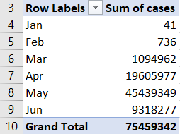
You would see your Pivot Table changing to following table (shown below). From this Pivot table we can answer our query which is "what is total number of US cases by month".
Sigma Values has lot of options, By default Excel does sum of values in the Pivot Table.. But we can ask it to do average, count, Min, Max and many others. Let us do one more example. This time we will do average number of cases in a month for each month.
Example: Problem statement: Show me the average number of cases by each month in USA
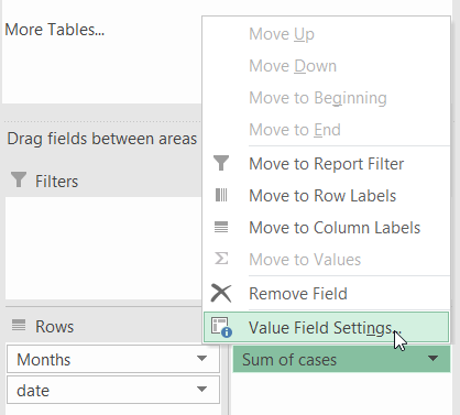
To do that click on "Sum of cases" and then click on "Value Field Settings" as shown below.
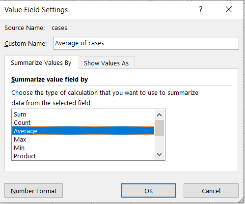
In the new pop up (shown below) select "Average". and click ok.
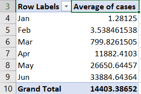
You should see a table as shown below. Below table shows average number of cases per day in each month.As shown below, the average number of cases per day kept on increasing in each month.
How to use filters in Pivot Tables in Excel
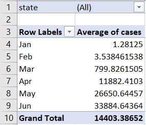
Filters help us slice the data further. Let us select "state" as one of the filters in our Pivot table. To do that drag the "state" field and drop in to the "Filters" column as shown below. Now we can analyze our data by each state.
Now you would see "state" column in your Pivot Table as one of filters as shown below.
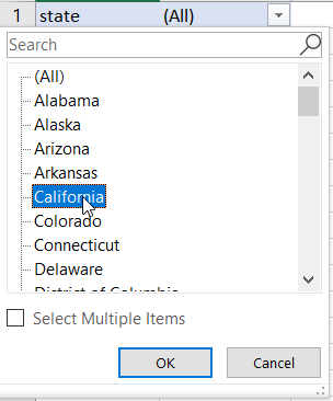
Now click on "state" drop down menu. You would see following dialog box. Let us select "California" as our state filter and click ok. That means, Data will be shown only for state "California".
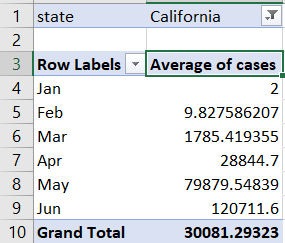
You should see the Pivot Table changed to following.
Wrap Up!
I hope you would find this tutorial useful.