How To Calculate Stocks Support And Resistance Using Clustering
In this notebook, I will show you how to calculate Stocks Support and Resistance using different clustering techniques.
Stock Data - I have stocks data in mongo DB. You can also get this data from Yahoo Finance for free.
MongoDB Python Setup
import pymongo
from pymongo import MongoClient
client_remote = MongoClient('mongodb://localhost:27017')
db_remote = client_remote['stocktdb']
collection_remote = db_remote.stock_data
Get Stock Data From MongoDB
I will do this analysis using last 60 days of Google data.
mobj = collection_remote.find({'ticker':'GOOGL'}).sort([('_id',pymongo.DESCENDING)]).limit(60)
Prepare the Data for Data Analysis
I will be using Pandas and Numpy for the data manipulation. Let us first get the data from Mongo Cursor object to Python list.
prices = []
for doc in mobj:
    prices.append(doc['high'])
Stocks Support and Resistance Using K-Means Clustering
import numpy as np
import pandas as pd
import matplotlib.pyplot as plt
from sklearn.cluster import AgglomerativeClustering
For K means clustering, we need to get the data in to Numpy array format.
X = np.array(prices)
For K means clustering, K which means number of clusters is very important. We can find the optimal K using the Knee plot as shown below.
from sklearn.cluster import KMeans
import numpy as np
from kneed import KneeLocator

sum_of_sq_distances = []
K = range(1,10)
for k in K:
    km = KMeans(n_clusters=k)
    km = km.fit(X.reshape(-1,1))
    sum_of_sq_distances.append(km.inertia_)
kn = KneeLocator(K, sum_of_sq_distances,S=1.0, curve="convex", direction="decreasing")
kn.plot_knee()
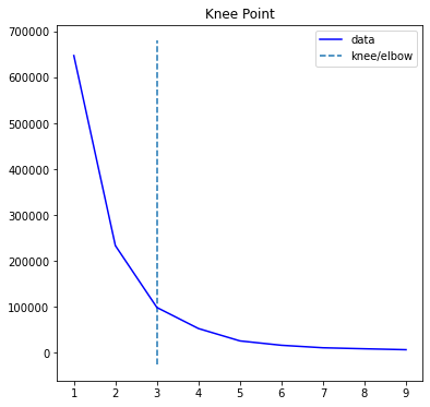
Let us check the value of K using kn.knee
kn.knee
kmeans = KMeans(n_clusters= kn.knee).fit(X.reshape(-1,1))
c = kmeans.predict(X.reshape(-1,1))
min_and_max = []
for i in range(kn.knee):
    min_and_max.append([-np.inf,np.inf])
for i in range(len(X)):
    cluster = c[i]
    if X[i] > min_and_max[cluster][0]:
        min_and_max[cluster][0] = X[i]
    if X[i] < min_and_max[cluster][1]:
        min_and_max[cluster][1] = X[i]
Let us check the min and max values of our clusters.
min_and_max
There are 3 clusters shown above, every cluster has max and min value.
At the writing of this notebook, Google stock price is 2687.98 (high of day) which happens to be 52 week high as well. Therefore based on the above clusters, we can say that 2687.98 is the resistance and next support level is 2508.0801. The next levels of support are 2461.9099, 2365.55 2357.02, 2239.4399.
Remember these support and resistances will change depending upon the range of data and value of Clustering parameter K.
Stocks Support and Resistance Using Agglomerative Clustering
mobj = collection_remote.find({'ticker':'GOOGL'}).sort([('_id',pymongo.DESCENDING)]).limit(60)
prices = []
for doc in mobj:
    prices.append(doc['high'])
Another approach that can be used is Agglomerative Clustering which is hierarchical clustering.
Agglomerative clustering is a bottoms up approach which merges child clusters to find out the big clusters of data.
I have found Aggloerative to be useful on stocks rolling data.
Let us create a rolling data of 20 days each for both calculating max and min values.
df = pd.DataFrame(prices)
max = df.rolling(20).max()
max.rename(columns={0: "price"},inplace=True)
min = df.rolling(20).min()
min.rename(columns={0: "price"},inplace=True)
Below step is required to prepare the data in two column format.
maxdf = pd.concat([max,pd.Series(np.zeros(len(max))+1)],axis = 1)
mindf = pd.concat([min,pd.Series(np.zeros(len(min))+-1)],axis = 1)
maxdf.drop_duplicates('price',inplace = True)
mindf.drop_duplicates('price',inplace = True)
Let us use n_clusters =3 value for our number of clusters.
F = maxdf.append(mindf).sort_index()
F = F[ F[0] != F[0].shift() ].dropna()

# Create [x,y] array where y is always 1
X = np.concatenate((F.price.values.reshape(-1,1),
                    (np.zeros(len(F))+1).reshape(-1,1)), axis = 1 )

cluster = AgglomerativeClustering(n_clusters=3,
          affinity='euclidean', linkage='ward')
cluster.fit_predict(X)
F['clusters'] = cluster.labels_

F2 = F.loc[F.groupby('clusters')['price'].idxmax()]

# Plotit
fig, axis = plt.subplots()
for row in F2.itertuples():

    axis.axhline( y = row.price,
            color = 'green', ls = 'dashed' )

axis.plot( F.index.values, F.price.values )
plt.show()
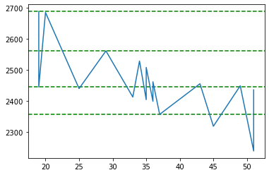
Let us plot our clusters now. As shown below, there are 2 clusters found. If we take in to account the todays closing price of Google which is 2638.00, we can say that 2687.98 is the resistance and 2357.02 is the support.
F2
One thing to notice here is that, there are only 2 clusters at price 2357.02 which is not that many. To see if we can find more number of clusters either we have to increase our number of price points in our source data or increase the number of clusters, or make our rolling window smaller.
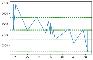
Let us increase the number of clusters to 5 and see what happens.
F = maxdf.append(mindf).sort_index()
F = F[ F[0] != F[0].shift() ].dropna()

# Create [x,y] array where y is always 1
X = np.concatenate((F.price.values.reshape(-1,1),
                    (np.zeros(len(F))+1).reshape(-1,1)), axis = 1 )

cluster = AgglomerativeClustering(n_clusters=5,
          affinity='euclidean', linkage='ward')
cluster.fit_predict(X)
F['clusters'] = cluster.labels_

F2 = F.loc[F.groupby('clusters')['price'].idxmax()]

# Plotit
fig, axis = plt.subplots()
for row in F2.itertuples():

    axis.axhline( y = row.price,
            color = 'green', ls = 'dashed' )

axis.plot( F.index.values, F.price.values )
plt.show()
F2
Ok this time around we got more number of clusters at price 2239.43 which is quite far from todays closing price of 2638. However the resistance number looks good of 2687.98 based on 3 clusters.
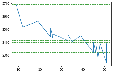
Let us make our rolling window smaller. Instead of 20 days let us make it 10 days.
df = pd.DataFrame(prices)
max = df.rolling(10).max()
max.rename(columns={0: "price"},inplace=True)
min = df.rolling(10).min()
min.rename(columns={0: "price"},inplace=True)
maxdf = pd.concat([max,pd.Series(np.zeros(len(max))+1)],axis = 1)
mindf = pd.concat([min,pd.Series(np.zeros(len(min))+-1)],axis = 1)
maxdf.drop_duplicates('price',inplace = True)
mindf.drop_duplicates('price',inplace = True)
F = maxdf.append(mindf).sort_index()
F = F[ F[0] != F[0].shift() ].dropna()

# Create [x,y] array where y is always 1
X = np.concatenate((F.price.values.reshape(-1,1),
                    (np.zeros(len(F))+1).reshape(-1,1)), axis = 1 )

cluster = AgglomerativeClustering(n_clusters=5,
          affinity='euclidean', linkage='ward')
cluster.fit_predict(X)
F['clusters'] = cluster.labels_

F2 = F.loc[F.groupby('clusters')['price'].idxmax()]

# Plotit
fig, axis = plt.subplots()
for row in F2.itertuples():

    axis.axhline( y = row.price,
            color = 'green', ls = 'dashed' )

axis.plot( F.index.values, F.price.values )
plt.show()
F2
Ok this data looks much better. We got a Google resistance around 2687.98 and support around 2399.03 and 2412.8799 which is quite close to say that support is around 2400.
Related Notebooks
- TTM Squeeze Stocks Scanner Using Python
- Pandas Datareader To Download Stocks Data From Google And Yahoo Finance
- Calculate Implied Volatility of Stock Option Using Python
- How to do SQL Select and Where Using Python Pandas
- Calculate Stock Options Max Pain Using Data From Yahoo Finance With Python
- How to Generate Embeddings from a Server and Index Them Using FAISS with API
- Pandas How To Sort Columns And Rows
- How to Visualize Data Using Python - Matplotlib
- How To Analyze Data Using Pyspark RDD