In this notebook, we will go over the text analysis of Stock tweets. This data has been scraped from stocktwits. I will use Python Pandas, Python library WordCloud and NLTK for this analysis. If you want to know more about Pandas, check my other notebooks on Pandas https://www.nbshare.io/notebooks/pandas/
Let us import the necesary packages.
import re
import random
import pandas as pd
import matplotlib.pyplot as plt
import seaborn as sns
%matplotlib inline
from plotly import graph_objs as go
import plotly.express as px
import plotly.figure_factory as ff
import json
from collections import Counter

from PIL import Image
from wordcloud import WordCloud, STOPWORDS, ImageColorGenerator


import nltk
from nltk.corpus import stopwords

import os
import nltk

import warnings
warnings.filterwarnings("ignore")
Let us check the data using Unix cat command.
!head -2 stocktwits.csv
Let us take a peak in to our data.
df = pd.read_csv('stocktwits.csv')
df.head()
As we see above, for each stock we have a tweet , sentiment, number of followers and date of stock tweet.
df.shape
Check if there are any 'na' values in data with df.isna(). We see below, there is no 'na' in data.
df.isna().any()
Check if there are any 'null' in data with df.isnull() command. As we see below, there are no null values in data.
df.isnull().any()
There are no null Values in the test set
Let us look at the distribution of tweets by stocks.
stock_gp = df.groupby('ticker').count()['message'].reset_index().sort_values(by='message',ascending=False)
stock_gp.head(5)
plt.figure(figsize=(12,6))
g = sns.distplot(stock_gp['message'],kde=False)
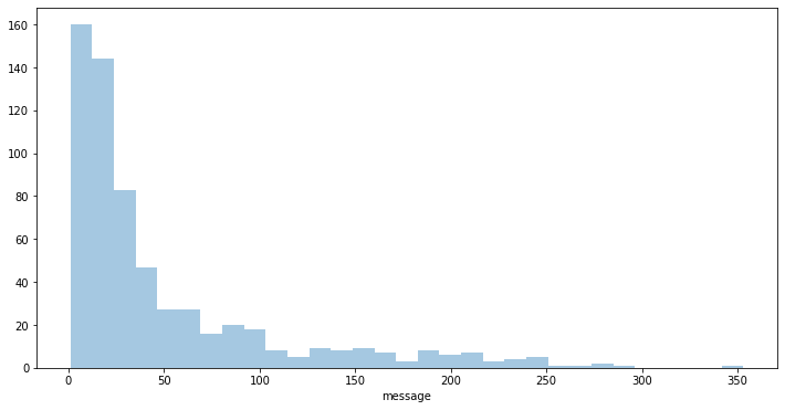
X-axis in the above plot shows the number of messages. Every bar represents a ticker.
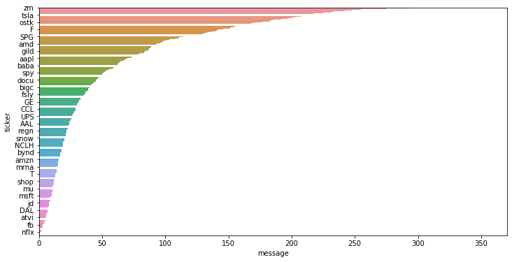
There is another way to plot which is bar plot (shown below) that will give us some more information about the stocks and their tweets. Note in the below plot, only few labels have been plotted, otherwise the y-axis will be cluttered with the labels if plot all of them.
import matplotlib.ticker as ticker
plt.figure(figsize=(12,6))
ax = sns.barplot(y='ticker', x='message', data=stock_gp)
ax.yaxis.set_major_locator(ticker.MultipleLocator(base=20))
Lets look at the distribution of tweets by sentiment in the data set.
temp = df.groupby('sentiment').count()['message'].reset_index().sort_values(by='message',ascending=False)
temp.style.background_gradient(cmap='Greens')
As we can see the data is skewed towards Bullish sentiments which is not surprising given the fact that since mid of 2020 market has been in uptrend.
df['words'] = df['message'].apply(lambda x:str(x.lower()).split())
top = Counter([item for sublist in df['words'] for item in sublist])
temp = pd.DataFrame(top.most_common(20))
temp.columns = ['Common_words','count']
temp.style.background_gradient(cmap='Blues')
Most of these words shown above are stop words. Let us remove these stop words first.
def remove_stopword(x):
    return [y for y in x if y not in stopwords.words('english')]
df['words'] = df['words'].apply(lambda x:remove_stopword(x))
top = Counter([item for sublist in df['words'] for item in sublist])
temp = pd.DataFrame(top.most_common(20))
temp.columns = ['Common_words','count']
temp.style.background_gradient(cmap='Blues')
Let us now plot the word clouds using Python WordCloud library.
def plot_wordcloud(text, mask=None, max_words=200, max_font_size=50, figure_size=(16.0,9.0), color = 'white',
                   title = None, title_size=40, image_color=False):
    stopwords = set(STOPWORDS)
    more_stopwords = {'u', "im"}
    stopwords = stopwords.union(more_stopwords)

    wordcloud = WordCloud(background_color=color,
                    stopwords = stopwords,
                    max_words = max_words,
                    max_font_size = max_font_size,
                    random_state = 42,
                    width=400,
                    height=400,
                    mask = mask)
    wordcloud.generate(str(text))

    plt.figure(figsize=figure_size)
    if image_color:
        image_colors = ImageColorGenerator(mask);
        plt.imshow(wordcloud.recolor(color_func=image_colors), interpolation="bilinear");
        plt.title(title, fontdict={'size': title_size,
                                  'verticalalignment': 'bottom'})
    else:
        plt.imshow(wordcloud);
        plt.title(title, fontdict={'size': title_size, 'color': 'black',
                                  'verticalalignment': 'bottom'})
    plt.axis('off');
    plt.tight_layout()
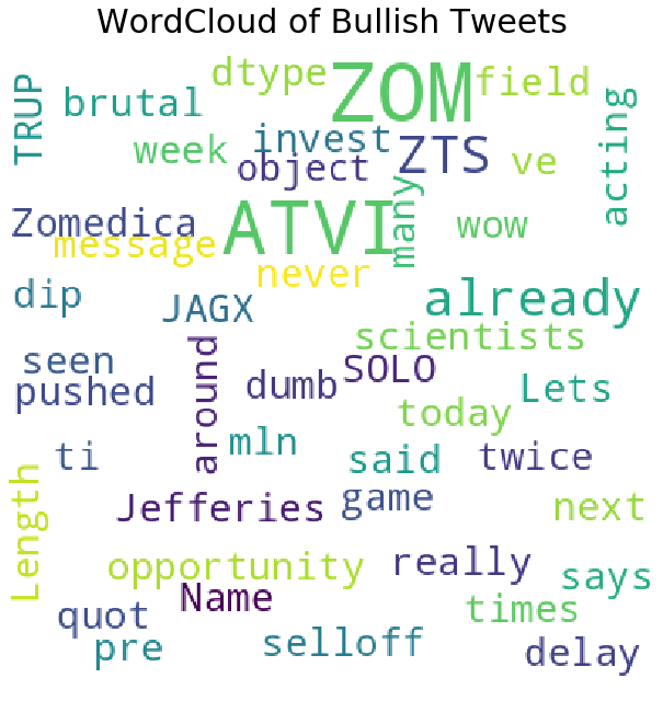
Let us first plot the word clouds of Bullish tweets only.
plot_wordcloud(df[df['sentiment']=="Bullish"]['message'],mask=None,color='white',max_font_size=50,title_size=30,title="WordCloud of Bullish Tweets")
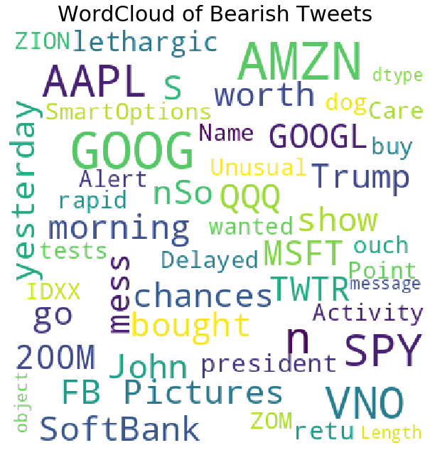
Ok let us plot WordCloud now for Bearish tweets.
plot_wordcloud(df[df['sentiment']=="Bearish"]['message'],mask=None,color='white',max_font_size=50,title_size=30,title="WordCloud of Bearish Tweets")
Related Notebooks
- Stock Sentiment Analysis Using Autoencoders
- Time Series Analysis Using ARIMA From StatsModels
- Tweet Sentiment Analysis Using LSTM With PyTorch
- Polynomial Interpolation Using Python Pandas Numpy And Sklearn
- Select Pandas Dataframe Rows And Columns Using iloc loc and ix
- Covid 19 Curve Fit Using Python Pandas And Numpy
- How to do SQL Select and Where Using Python Pandas
- Data Analysis With Pyspark Dataframe
- Pandas Read and Write Excel File