This tutorial explores image classification in PyTorch using state-of-the-art computer vision models. The dataset used in this tutorial will have 3 classes that are very imbalanced. So, we will explore augmentation as a solution to the imbalance problem.
Data used in this notebook can be found at https://www.nbshare.io/blog/datasets/
import os
import random
import numpy as np
import pandas as pd
from PIL import Image
from sklearn.metrics import accuracy_score
from sklearn.model_selection import train_test_split
import torch
from torch import nn
import torch.nn.functional as F
from torch.utils.data import Dataset, DataLoader, WeightedRandomSampler
from torchvision import datasets, models
from torchvision import transforms
import matplotlib.pyplot as plt
Setting the device to make use of the GPU.
device = torch.device("cuda" if torch.cuda.is_available() else "cpu")
device
Identifying the data paths.
data_dir = "images/"
labels_file = "images_labeled.csv"
Since the labels are in a CSV file, we use pandas to read the file and load it into a DataFrame
labels_df = pd.read_csv(labels_file)
labels_df.head()
As shown, we have 3 classes that are imbalanced.
labels_df["Category"].value_counts()
Creating numerical IDs for each class. The following list and dictionary are used for converting back and forth between labels and IDs.
id2label = ["Technical", "Others", "News"]
label2id = {cl:idx for idx, cl in enumerate(id2label)}
We use pandas to split the data into an 80-20 split.
train_labels_df, test_labels_df = train_test_split(labels_df, test_size = 0.2)
train_image_names = list(train_labels_df["Image Name"])
train_image_labels = list(train_labels_df["Category"])
test_image_names =  list(test_labels_df["Image Name"])
test_image_labels =  list(test_labels_df["Category"])
train_image_names[:5]
print("Train set size:", len(train_labels_df),
      "\nTest set size:", len (test_labels_df))
The solution we follow in this tutorial for data imbalance is to create a random weighted sampler that, in each batch, takes approximately the same number of images from each class. It does so by using replacement sampling with the inferior classes.
However, that alone is not enough. Since there will be replacement in sampling (meaning that the same image can repear twice in a batch), we need to perform augmentation on all images to add some differences.
This is performed using PyTorch "transforms".
For both training and test sets, we will apply the following transformations to create augmented versions of the images:
transform_dict = {'train': transforms.Compose([
        transforms.RandomResizedCrop(224),
        transforms.RandomHorizontalFlip(),
        transforms.ToTensor(),
        transforms.Normalize([0.485, 0.456, 0.406], [0.229, 0.224, 0.225])
    ]),
    'test': transforms.Compose([
        transforms.Resize((224, 224)),
        transforms.CenterCrop(224),
        transforms.ToTensor(),
        transforms.Normalize([0.485, 0.456, 0.406], [0.229, 0.224, 0.225])
    ]),}
class ImageDS(Dataset):
    def __init__(self, data_dir, image_names, labels, transformations):
        self.image_names = image_names
        self.labels = [label2id[label] for label in labels]
        self.transforms = transformations
        self.data_dir = data_dir
        self.img_paths = [os.path.join(self.data_dir, name)
                         for name in self.image_names]

    def __len__(self):
        return len(self.img_paths)

    def __getitem__(self, idx):
        """
            Opens an image and applies the transforms.
            Since in the dataset some images are PNG and others are JPG,
              we create an RGB image (no alpha channel) for consistency.
        """
        img = Image.open(self.img_paths[idx])
        label = self.labels[idx]
        rgbimg = Image.new("RGB", img.size)
        rgbimg.paste(img)
        rgbimg = self.transforms(rgbimg)

        return rgbimg, label
Initializing the Datasets
train_ds = ImageDS(data_dir, train_image_names, train_image_labels, transform_dict['train'])
test_ds = ImageDS(data_dir, test_image_names, test_image_labels, transform_dict['test'])
Plotting an image to verify the changes. As shown, the image is cropped into a 224x224 square as intended.
plt.imshow(train_ds[0][0].permute(1, 2, 0))
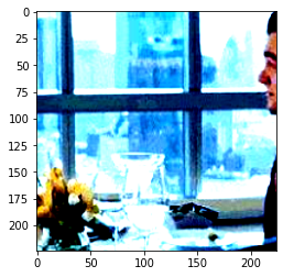
The corresponding label:
id2label[train_ds[0][1]]
Random Weighted Sampling and DataLoaders
PyTorch provides an implementation for random weighted sampling using this class:
WeightedRandomSampler()This class takes 2 parameters to create the sampler: the weights of each instance of each class, and the size of the dataset. We calculate the weights and create the sampler using this function:
def create_weighted_sampler(ds):
    class_prob_dist = 1. / np.array(
        [len(np.where(np.array(ds.labels) == l)[0]) for l in np.unique(ds.labels)])
    classes = np.unique(ds.labels)
    class2weight = {cl:class_prob_dist[idx] for idx, cl in enumerate(classes)}
    weights = [class2weight[l] for l in ds.labels]
    return WeightedRandomSampler(weights, len(ds))
Initializing samplers:
train_sampler = create_weighted_sampler(train_ds)
test_sampler = create_weighted_sampler(test_ds)
Finally, we use those samplers while creating the DataLoaders. That way the DataLoaders are ready to provide balanced data.
train_dl = DataLoader(train_ds, batch_size=16, sampler = train_sampler)
test_dl = DataLoader(test_ds, batch_size=16, sampler=test_sampler)
dataloaders = {"train": train_dl, "test": test_dl}
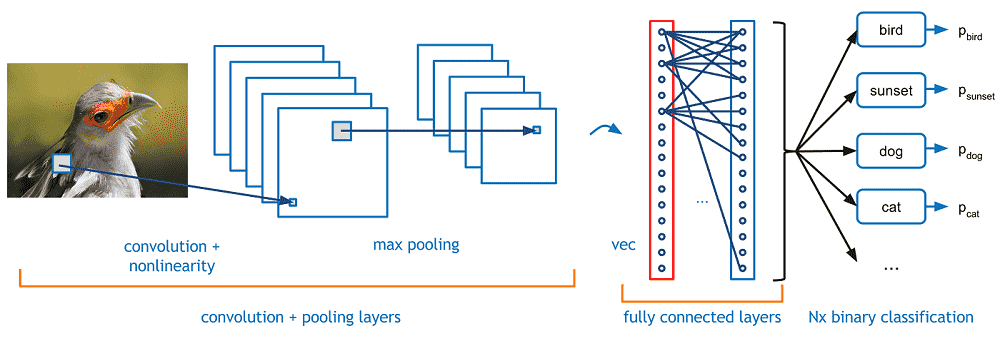
The following is a simple CNN model. We use ResNet as the main model in this tutorial, but you can use the CNN below instead by initializing the model to CNN().
class CNN(nn.Module):
    def __init__(self):
        super().__init__()
        self.conv1 = nn.Conv2d(3, 6, 5)
        self.pool = nn.MaxPool2d(2, 2)
        self.conv2 = nn.Conv2d(6, 16, 5)
        self.fc1 = nn.Linear(44944, 120)
        self.fc2 = nn.Linear(120, 84)
        self.fc3 = nn.Linear(84, 10)

    def forward(self, x):
        x = self.pool(F.relu(self.conv1(x)))
        x = self.pool(F.relu(self.conv2(x)))
        x = torch.flatten(x, 1) # flatten all dimensions except batch
        x = F.relu(self.fc1(x))
        x = F.relu(self.fc2(x))
        x = self.fc3(x)
        return x
To choose the CNN, run this cell and not the one below it:
model = CNN()
model = model.to(device)
model
Here, we use ResNet-101 as the model:
model = models.resnet101(pretrained=True)
num_ftrs = model.fc.in_features
# for param in model.parameters(): # Uncomment these 2 lines to freeze the model except for the FC layers.
    # param.requires_grad = False
model.fc = nn.Linear(num_ftrs, 3)
Sending model to device
model = model.to(device)
Initializing the criterion and optimizer:
criterion = nn.CrossEntropyLoss()
optim = torch.optim.Adam(model.parameters(), lr = 1e-3)
training_losses = []
test_losses = []
for epoch in range(15):  # loop over the datasets multiple times
    for phase in ["train", "test"]: # loop over train and test sets separately
        if phase == 'train':
            model.train()  # Set model to training mode
        else:
            model.eval()   # Set model to evaluate mode
        running_loss = 0.0
        for i, data in enumerate(dataloaders[phase], 0): # loop over dataset
            # get the inputs; data is a list of [inputs, labels]
            inputs, labels = data

            inputs = inputs.to(device) # loading data to device
            labels = labels.to(device)
            # zero the parameter gradients
            optim.zero_grad()
            # forward + backward + optimize
            outputs = model(inputs)
            loss = criterion(outputs, labels)
            _, preds = torch.max(outputs, 1)
            loss.backward()

            # Performing gradient clipping to control our weights
            torch.nn.utils.clip_grad_norm_(model.parameters(), 0.7)
            optim.step()
            if phase == 'train':
                training_losses.append(loss.item())
            else:
                test_losses.append(loss.item())
            # print statistics
            running_loss += loss.item()
            print_freq = 10
            if i % print_freq == 0:    # print every 10 mini-batches
                print('%s: [%d, %5d] loss: %.3f' %
                    (phase, epoch + 1, i + 1, running_loss / print_freq))
                running_loss = 0.0

print('Finished Training')
plt.plot(training_losses)
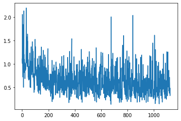
plt.plot(test_losses)
plt.ylim([0, 3])
plt.show()
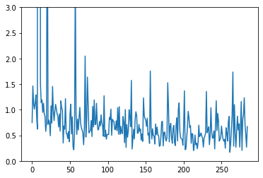
We can observe from the training and the losses that the model learned, although it was noisy.
We find the accuracy by predicting the test set:
preds_total = []
for i, data in enumerate(test_dl, 0):
    # get the inputs; data is a list of [inputs, labels]
    inputs, labels = data

    inputs = inputs.to(device)
    labels = labels.to(device)
    # zero the parameter gradients
    optim.zero_grad()

    # obtaining predictions
    with torch.set_grad_enabled(False):
        logits = model(inputs)
        preds = torch.argmax(logits, 1)
        print(i)
        preds_total += preds.to('cpu').tolist()
print(type(preds_total), len(preds_total))
print(type(test_ds.labels), len(test_ds.labels))
accuracy_score(preds_total, test_ds.labels)
The accuracy is ~45%
Despite using a SOTA model, advanced image processing, and good imbalance solutions, the accuracy of this 3 class task is relatively low. There are 2 main problems we can observe:
There are many incorrect labels in the data. This adds noise in the learning process and confuses the model, preventing it to learn from many instances. The graphs of the loss demonstrate this problem, where the plot increases and decreases sharply. The solution is to recheck the labels.
The 2nd problem I observe is the content of the "Other" class. It is always better to avoid including an "other" class in image classification, or at least to keep the instances in the "other" class relatively similar. The "other" images in the data are very random, making it difficult to detect. The solution is to either try training without this class, or to improve the quality of the images in this class. That way, the model is not very confused about the content of this class.
To further validate the perforamance, we predict the labels for random images in the test set:
# Get a random test image
random_id = random.randint(0, len(test_labels_df))
img_name, lbl = test_labels_df.iloc[random_id]
img_name, lbl
img = Image.open(os.path.join(data_dir, img_name))
rgbimg = Image.new("RGB", img.size)
rgbimg.paste(img)
img = transform_dict['test'](rgbimg)
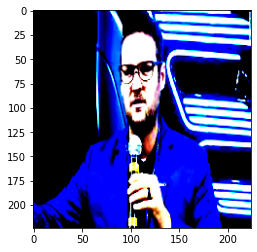
plt.imshow(img.permute(1,2,0))
# First, send the image to device
img = img.to(device)
# Feed the image to the model
logits = model(img[None, ...])
# Get the class with the highest score
_, preds = torch.max(logits, 1)
pred = preds.item()
id2label[pred]
pred == label2id[lbl]
However, the model is correct for the shown example above, as it predicted category "Others" because it is neither News nor stock chart.
Related Notebooks
- Generating Image Scribbles with Stable Diffusion and ControlNet
- Activation Functions In Artificial Neural Networks Part 2 Binary Classification
- Stock Sentiment Analysis Using Autoencoders
- Demystifying Stock Options Vega Using Python
- Calculate Implied Volatility of Stock Option Using Python
- Stock Tweets Text Analysis Using Pandas NLTK and WordCloud
- Plot Stock Options Vega Implied Volatility Using Python Matplotlib
- Calculate Stock Options Max Pain Using Data From Yahoo Finance With Python
- Crawl Websites Using Python